In this chapter, we will cover the basics of estimation in Stan. In particular, this chapter will start from a basic linear regression in Stan, and then quickly move to more specilized topics in nonlinear estimation. While in practice you are unlikely to want to use Stan for the type of aggregate- or individual-level estimation discussed in this chapter, it constitutes an important stepping stone in familiarizing yourself with Stan and Bayesian estimation more generally. Aggregate models also constitute an important point of reference to which more complex hierarchical models—covered in chapter III—can be compared. Indeed, it is always a good idea to start from a simple model, and to then increase its complexity step-by-step towards your preferred specification. Although it may sound paradoxical, this can save you a lot of time in the end, especially when highly nonlinear hierarchical models on largish datasets may run for hours or days on end.
3.1 Basics of Stan coding
3.1.1 About Stan
Stan is a very versatile programme for Bayesian analysis written in C++. It can be launched from a number of different platforms, including \(R\) and the command prompt. Analysis files are written in text editors, and the programmes need to be compiled before they can be run. Always keep the Stan user manual close by to look up the best way of implementing a programme https://mc-stan.org/users/documentation/). Also consult the online resources on implemented functions https://mc-stan.org/docs/2_21/functions-reference/), and if need be, the user community website https://discourse.mc-stan.org/).
At the time of writing, there are two ways of launching Stan from R. Rstan works like a standard R package. CmdStanR works as an R interface to communicate with the terminal. There are pros and cons to each method. Rstan will look more familiar to R users, especially when it comes to post-processing of estimation results. It also makes it easier to set and control starting values, and the experience is smoother, in that Rstan tends to throw fewer (and more meaningful) errors. CmdStanR, however, has the advantage that it is quite a bit faster. It is also much lighter in terms of memory use—a decisive quality if you want to estimate large models, which in Rstan frequently lead to crashes. While at the time of writing there are other differences between the two modes of operations, these are subject to rapid change, and are thus not described here. In this tutorial, I will use CmdStanR throughout. You can find detailed instructions on the installation and a guide to get you started at https://mc-stan.org/cmdstanr/articles/cmdstanr.html
3.1.2 The structure of a Stan model
The basic structure of a Stan model looks as follows:
Show the R code
functions {// ... self-defined functions (optional) ...}data {// ... all data need to be specified ...}transformed data {// ... data can be transformed here (optional) ...}parameters {// ... declare all parameters to be used ...}transformed parameters {// ... transform parameters (optional) ...}model {// ... define priors and write model ...}generated quantities {// ... post-estimation commands (optional) ...}
The data block, the parameters block, and the model block are compulsory. The other blocks are optional, but will often turn out to be useful. We will explore the use of different statements within the blocks progressively as we move through these notes. The different blocks present some overlaps. For instance, one can declare variables in the parameters block, the transformed parameters block, in the model block, or even the generated quantities block. However, variables declared in the model block are only available locally in that block, and variables declared in generated quantities are not available in any earlier blocks. Variables declared in the parameters or in the transformed parameters block, on the other hand, are available globally. E.g., they can be used directly in the model block without the need to declare them again.
3.2 Linear regression
3.2.1 A simple regression
In this section, we will examine a simple linear regression model, and learn how to programme it in Stan. Take the following equation: \[
y_n = \alpha + \beta x_n + \epsilon_n,
\] where \(n\) indicates a single observation, and \(\epsilon_n \sim \mathcal{N}(0,\sigma)\) (NOTE: I follow the convention in Stan to write the standard deviation in the distribution, instead of the variance). This equation can be rewritten as follows: \[
y_n - (\alpha + \beta x_n) \sim \mathcal{N}(0,\sigma) ,
\] or indeed as \[
y_n \sim \mathcal{N}(\alpha + \beta x_n,\sigma).
\] The latter form is typically used to code regression models in Stan.
To make the problem more interesting, let \(y = ce\) be a certainty equivalent, and \(x = p\) the probability of winning provided by the wager. The following implements a Stan model regressing the certainty equivalent on the probability of winning the prize:
Show the R code
data{int<lower=0> N;vector[N] ce;vector[N] p;}parameters{real alpha;real beta;real<lower=0> sigma;}model{ ce ~ normal(alpha + beta * p , sigma) ;}
A few comments are in place. The statement <lower = 0> indicates that a variable is limited below at 0. This is optional for data, where it serves mostly as a check on the data one imports. It is essential for some variables, such as \(\sigma\) in the example above, since the programme may otherwise attempt to sample negative values. Certain data need to be coded as integers, or else they will be rejected by Stan. For instance, this always applies to the sample size \(N\), and we will see other examples in due time. The data are imported as vectors, which—where possible—has computational advantages and speeds up the sampling. Alternatively, the model line could be rewritten using a loop:
The latter way of writing the model is slightly slower. However, it provides additional flexibility in contexts where matrix notation cannot be used, e.g. because of the use of powers, or because of difficulties in matching the dimensions of parameter and data matrices in hierarchical models. Finally, you should notice that I have not specified any priors. This means that Stan will automatically set the prior for the parameters to a uniform distribution over the whole support of the parameters. We willll return to priors later.
Let us now go ahead and estimate the model. We can use the data of Bouchouicha and Vieider (2017), experiment 1. We will start by creating a new dataset to send to Stan. This helps because Stan hates missing values, even in variables it does not use. It is also a chance to rename and transform variables to get them into the appropriate format. In this instance, it is convenient to normalize the CE by dividing it by the prize of the wager (try running it without the normalization to convince yourself of this):
Show the R code
bv <-read.csv(file="data/data_BV_exp1.csv")# creates data to send to StanstanD <-list(N =nrow(bv), ce = bv$ce/bv$high,p = bv$prob )# compile the Stan programme:sr <-cmdstan_model("stancode/agg_normal.stan")# run the programme:nm <- sr$sample(data = stanD, seed =123, chains =4,parallel_chains =4,refresh=0,init=0,show_messages =TRUE,diagnostics =c("divergences", "treedepth", "ebfmi"))print(nm, c("alpha","beta","sigma"),digits =3)nm$save_object(file="stanoutput/agg_normal.Rds")
The coefficient \(\beta = 0.65\) can be interpreted as the slope of a neoadditive weighting function, \(w(p) = \alpha + \beta p\), capturing likelihood-insensitivity; the intercept can proxy for optimism (see Abdellaoui et al. (2011) for more appropriate indices, such as \(1 -\beta - 2*\alpha\)). The sd is the standard deviation of the posterior simulations, which is equivalent to a standard error in frequentist statistics, except that we can directly conclude that \(\beta\) has a 90% probability of falling between 0.627 and 0.681.
It may be interesting to determine the proportion of the overall variance in CEs explained by this simple model. One complication, however, is that the output contains the standard deviation of the error instead of the \(R^2\). This is easily solved using the definition of \(R^2\):
where \(\sigma^2_0\) is the variance of the model empty of covariates. In this case, I have obtained this measure simply from the data by using var(bv$ce_norm), and \(\sigma^2_1\) is the variance of the model estimated above. Technically, one could obtain \(\sigma_0\) from estimating a model empty of co-variates, and then derive an \(R^2\) measure that is itself an uncertain quantity. While properly Bayesian, this is rarely done in practice since it produces informational overload.
One can now use the posterior simulations obtained from the model in a variety of ways:
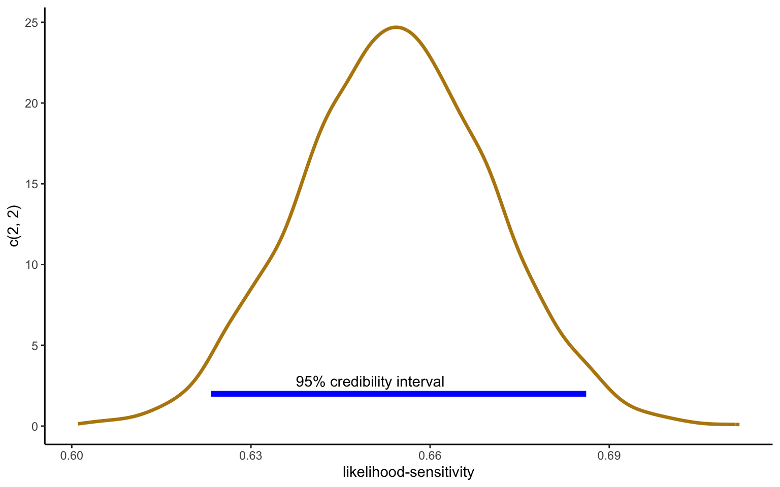
Figure 3.1: Slope parameter of linear regression of ce/x on p
The distribution in Figure 3.1 represents all the posterior draws of the parameter \(\beta\), which I refer to as likelihood-sensitivity. Note that in the Bayesian interpretation, it is indeed the parameter that is considered uncertain, while the data are treated as given. The blue line gives the 95% credibility interval (which in the symmetric case coincides with the 95% highest density interval), which gives the probability that the true parameter falls within the indicated range.
3.2.2 Multiple regression
We have so far regressed our CEs only on one single variable. It is, however, straightforward to extend this setup to multiple variables, e.g. by using the following code:
Show the R code
model{ce ~ normal(alpha + beta_p * p + beta_h * high , sigma) ;}
We now have expanded the code to include two independent variables (don’t forget to import the new variable in the data block, and to add the new parameter in the parameters block). However, one can see how this sort of coding can get old quicklyfor models with many independent variables, we will need to code a new model for every single specification we intend to use! A better way to go about it will thus be to code the regression coefficients as a vector. That is easily achieved with the following code:
I am now declaring an additional data point \(k\), which gives me the columns of the design matrix \(x\). The design matrix includes a column of 1s, so that I have furthermore dropped the intercept parameter \(\alpha\), with the first coefficient in \(\beta\) taking its place. Given that the model is written in matrix notation, \(\beta\) needs to be post-multiplied with the design matrix.
Show the R code
x <-model.matrix(~prob + high, data = bv)# creates data to send to StanstanD <-list(N =nrow(bv), k =ncol(x),ce = bv$ce/bv$high,x = x)# compile the Stan programme:sr <-cmdstan_model("stancode/agg_normal_multi.stan")# run programme:nm <- sr$sample(data = stanD, seed =123, chains =4,parallel_chains =4,refresh=0,init=0,show_messages =TRUE,diagnostics =c("divergences", "treedepth", "ebfmi"))print(nm, c("beta","sigma"),digits =3)nm$save_object(file="stanoutput/agg_normal_multi.Rds")
The coefficients obtained for probability and prize are difficult to compare directly, given the different scale of the prize. However, an interesting question may be how much more variance is explained once we add the prize over the regression on probabilities alone. The answer is not much. The total \(R^2\) of the model is now 0.6754313, which is not much higher than the one of the simple model above. This is the sense in which Bouchouicha and Vieider (2017) conclude that likelihood-distortions are much more important than outcome-distortions to account for behaviour!
3.2.3 A linearized dual-EU model
We have started making some inferences on the goodness of fit of different models using linear regression. We can, however, also estimate linearized versions of nonlinear models using linear regression techniques. For \(u(x) = x^r\), we can rewrite the EU model \(u(c) = pu(x)\) as \(c = u^{-1}(p) x\), which gives us a dual-EU model. We know that risk attitudes over probabilities tend to change rather radically as one moves from small to large probabilities, certainly when using CEs. A function that has often been used to capture this pattern is as follows: \[
\pi(p) = \frac{\delta p^\gamma}{\delta p^\gamma + (1-p)^\gamma}
\] The function is highly non-linear. It can, however, be reformulated in terms of log-odds as follows: \[
ln \left(\frac{\pi(p)}{1-\pi(p)} \right) = ln(\delta) + \gamma \, ln \left( \frac{p}{1-p} \right)
\] Note also that under dual-EU \(\pi(p) \triangleq \frac{ce - y}{x - y}\). This means that the left-hand side is fully defined in terms of the data. The right hand side has two parameters. Since these happen to be simply a slope and an intercept, we can estimate them using a simple linear regression.
In the code above, I use the transformed data block to obtain the measures of interest (alternatively, I could have created them in R and declared them as data). I also use the generated quantities block to recover \(\delta\)—the true quantity of interest, giving us optimism––-from the estimated intercept \(\alpha = ln(\delta)\), so that \(\delta = exp(\alpha)\). We can easily recover this parameter from the posterior including all the parameter uncertainty (note that this could also be done post-processing in R if need be). This is indeed a strength of the Bayesian approach: we can manipulate parameters in the posterior as we want, all the while carrying along all and any parameter uncertainty. Executing the programme and recovering and manipulating these quantities is left for your as an exercise.
3.3 Refinement of regression models
3.3.1 Robust regression
We have so far used the normal density in regressions, but nothing is special about the normal density. That is, we can simply replace that density by an alternative density of our choice. A fitting choice may be the Student-t density, which due to its fat tails is often used to implement robust regression. That is, the fat tails allow the distribution to discount outliers, thus making the results more robust to outlying observations. The following code implements such a regression with 2 degrees of freedom for the Student-t distribution:
x <-model.matrix(~ prob + high, data = bv)# creates data to send to StanstanD <-list(N =nrow(bv), k =ncol(x),ce = bv$ce/bv$high,x = x)# compile the Stan programme:sr <-cmdstan_model("stancode/agg_student.stan")# run programme:nm <- sr$sample(data = stanD, seed =123, chains =4,parallel_chains =4,refresh=0,init=0,show_messages =TRUE,diagnostics =c("divergences", "treedepth", "ebfmi"))print(nm, c("beta","sigma"),digits =3)nm$save_object(file="stanoutput/agg_student.Rds")
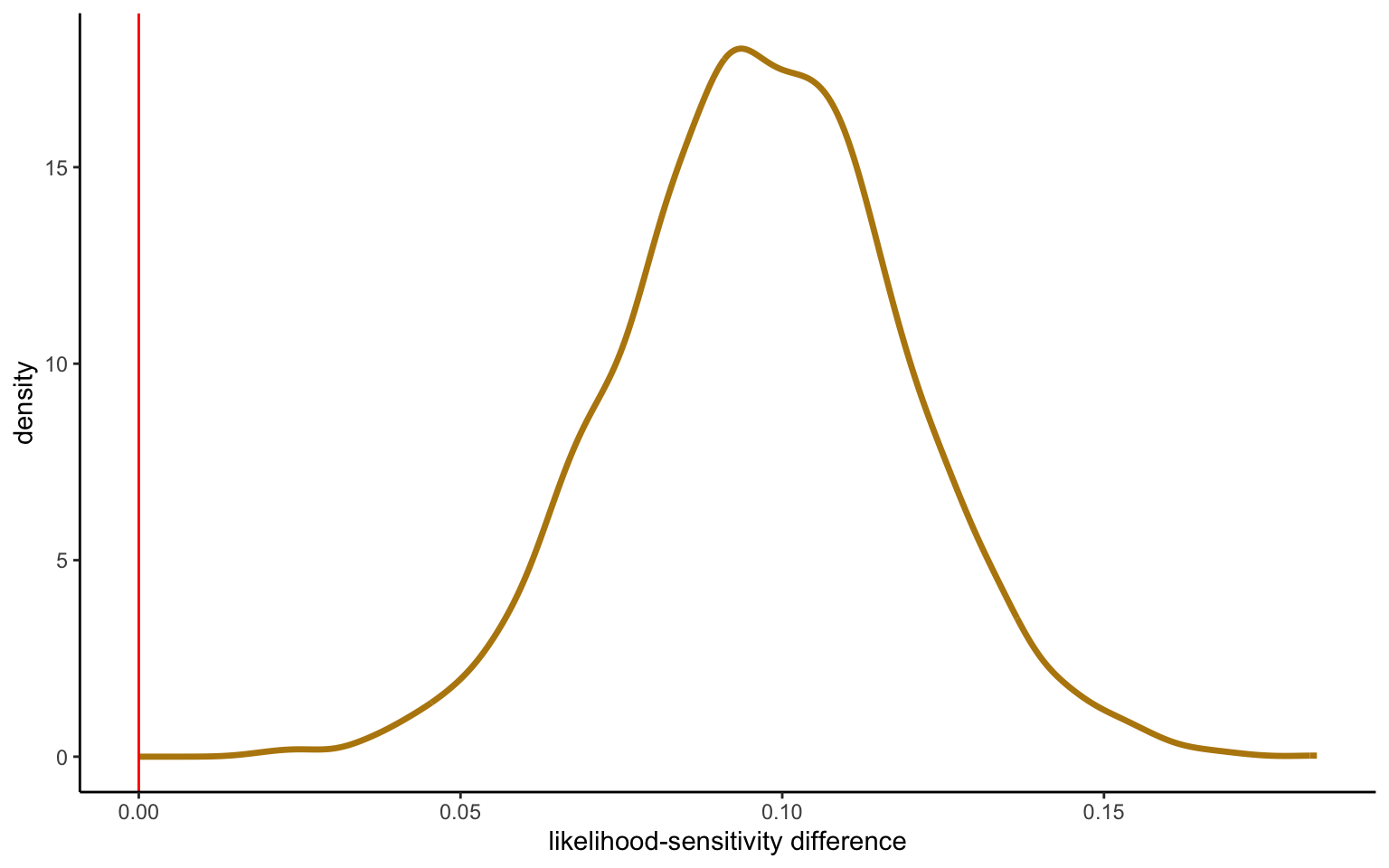
The parameters have changed rather significantly, with a lower intercept and larger slope/sensitivity. We can, indeed, test for this difference:
Figure 3.2: Slope difference from normal verus student-t distribution
The test for the difference is technically carried out by taking the difference of all the observations in the posterior simulations. One can then compare this difference to a benchmark of 0 (or some interval around 0 that can be justified as an acceptability region), and quantify how much of the probability mass lines up with the hypothesis. This is shown in Figure 3.2. In this case, virtually all the probability mass falls above 0, showing a significant difference between the two estimates. To test this, once could simply look at the probability mass falling above 0 (or above 0.03 or 0.05, depending on how one wants to conceive of the null hypothesis).
Differences in the estimates are not truly what we are interested in here. One could now go ahead and directly test for model performance (we will discuss how to do this at a later point). Another possibility may be to construct a model where the degrees of freedom are estimated endogenously. If outliers are indeed a problem, the degrees of freedom ought to be estimated to some low number. If this is not the case, we will get large degrees of freedom, and the distribution will approach the normal distribution (at infinity in theory, but starting already from about 10 for all practical purposes; see Kruschke (2013) for details). Here is the code implementing such a model:
x <-model.matrix(~prob + high, data = bv)# creates data to send to StanstanD <-list(N =nrow(bv), k =ncol(x),ce = bv$ce/bv$high,x = x)# compile the Stan programme:sr <-cmdstan_model("stancode/agg_student_end.stan")# run the programme:nm <- sr$sample(data = stanD, seed =123, chains =4,parallel_chains =4,refresh=0,init=0,show_messages =TRUE,diagnostics =c("divergences", "treedepth", "ebfmi"))print(nm, c("df","beta","sigma"),digits =3)saveRDS(nm,file="stanoutput/agg_student_end.Rds")
The degrees of freedom are estimated at 5, thus falling into a range where the student-t distribution differs substantially from the normal distribution. This vindicates the use of the student-t, and suggests that it would indeed perform better than a normal distribution in out-of-sample prediction. We will leave a test of this statement for a later chapter. Notice, however, that it is relatively low cost to move to a student-t distribution. This only costs one more parameter, which for most datasets is not an issue at the aggregate level. If the underlying distribution is truly normal, the student-t will reflect this automatically by estimating large degrees of freedom. If it is not, we have built a model that is resistant to outliers. Win-win.
3.3.2 Reparameterizing the model
Although mathematically equivalent, different ways of parameterizing a model can have a large impact on the convergence of a model in Stan. The details of this depend on how the Hamiltonian Monte Carlo simulation algorithm explores the parameter space. This is an issue to which we will have to return repeatedly in these notes. Here, I specifically discuss reparameterizing the regression matrix and coefficients. Although in the simple model above we did not encounter any problems, issues will quickly arise when we move to more complex models. This is especially true when several regression variables are (partially) colinear, which creates difficulties for the algorithm in exploring the parameter space. The solution will thus involve transforming the independent variables in a way as to be orthogonal.
For regression analysis, we will want to decompose the design matrix as follows: \(x = QR\), where \(Q\) is an orthogonal matrix, and \(R\) an upper triangular matrix, referred to, rather fittingly, as Q-R decomposition. Major commercial software typically performs this decomposition under the hood. Luckily, these days Stan allows us to directly implement this within the programme, without the need to first do the decomposition by hand in R, and later reconvert the parameters to the original scale. Most of the action happens within the transformed data block, with the model part integrating the regression on the orthogonal matrix. The generated quantities part is then used to transform the regression parameters back to the original scale:
Show the R code
data { int<lower=0> N;int<lower=0> k; matrix[N, k] x;vector[N] ce;}transformed data {matrix[N, k] Q_ast;matrix[k, k] R_ast;matrix[k, k] R_ast_inverse;// thin and scale the QR decomposition: Q_ast = qr_thin_Q(x) * sqrt(N - 1);R_ast = qr_thin_R(x) / sqrt(N - 1);R_ast_inverse = inverse(R_ast);}parameters {vector[k] gamma; // coefficients on Q_astreal<lower=0> sigma; // error scale}model {ce ~ normal(Q_ast * gamma , sigma); // likelihood}generated quantities {vector[k] beta;beta = R_ast_inverse * gamma; // coefficients on x}
You can convince yourself that the vector beta contains estimates identical to those obtained previously. Although in the present setup this does not (yet) make a difference, it is good practice to code any regression using the Q-R decomposition from the start. Otherwise, you risk to get stuck at some point without knowing why. Your estimations may also run much more slowly, which for large and complex models can become a real problem.
3.3.3 Introducing priors
Let us again use the example above. We can formulate priors as follows:
The parameter beta[1] represents the intercept in our regression model. The prior mean at 0 is chosen to be uninformative; the SD is chosen so as to give the parameter a wide berthgiven what we know about the quantities in the model, we would typically not expect it to be much above 0.3 or below -0.3, yet we have attributed substantial probability mass to the range from -1 to 1. Such priors are called mildly regularizing, inasmuch as they help the estimation algorithm to search in roughly the right range without imposing any strong prior opinions of where we would expect the estimates to fall.
The prior for beta[2] has been chosen to be somewhat more informative. We know from a large literature on likelihood-insensitivity that the parameter will typically fall below 1, and typical values may be between 0.6 and 0.8 (given a meta-analysis, one could use the posterior from the analysis as the prior for new estimations). At the same time, the SD is chosen to be somewhat more restrictive, while still providing enough wiggle room not to influence the final estimates too much. (Of course, you should always play around with the prior to make sure this is the case).
A more interesting question concerns what may happen if we choose a prior that is wildly inappropriate. Imagine we take a prior with mean 2 and SD 0.1, giving a negligible probability to the maximum likelihood estimate. This results in an estimate of 0.736 instead of 0.686. A distortion to be sure, but not a huge one, considering how far away and how overconfident the prior is. The reason is simply that the amount of data is easily enough to largely overwrite even a relatively strong and wildly inappropriate prior (i.e., the data will typically produce estimates with enough precision to counteract the narrow variance of the prior). As a general rule, the less data one has, the more impact the prior will havefor good or for bad. Priors should thus be chosen wisely, and one should examine the stability of the model to several assumptions about the prior to make sure that it does not unduly distort the results.
3.3.4 Informative priors on sparse stimuli
It may be interesting to see what happens when there are relatively little data to work with. It is in these cases that priors will unfold their true power. This may well be a bad thing, as happens when priors unduly influence the posterior estimates one obtains, possibly even without the analyst being aware of it. To see what might happen, we can run the same model as above on a much reduced dataset. For instance, let us select only one subject at random:
Show the R code
bv5 <- bv %>%filter(subject==5) x <-model.matrix(~ prob + high, data = bv)# creates data to send to StanstanD <-list(N =nrow(bv5), ce = bv5$ce/bv5$high,p = bv5$prob)# compile the Stan programme:sr <-cmdstan_model("stancode/agg_normal.stan")# run programme:nm <- sr$sample(data = stanD, seed =123, chains =4,parallel_chains =4,refresh=0,init=0,show_messages =TRUE,diagnostics =c("divergences", "treedepth", "ebfmi"))print(nm, c("alpha","beta","sigma"),digits =3)saveRDS(nm,file="stanoutput/agg_normal_s5.Rds")# run again with strong priorsr <-cmdstan_model("stancode/agg_normal_dp.stan")nm <- sr$sample(data = stanD, seed =123, chains =4,parallel_chains =4,refresh=0,init=0,show_messages =TRUE,diagnostics =c("divergences", "treedepth", "ebfmi"))print(nm, c("alpha","beta","sigma"),digits =3)saveRDS(nm,file="stanoutput/agg_normal_s5dp.Rds")
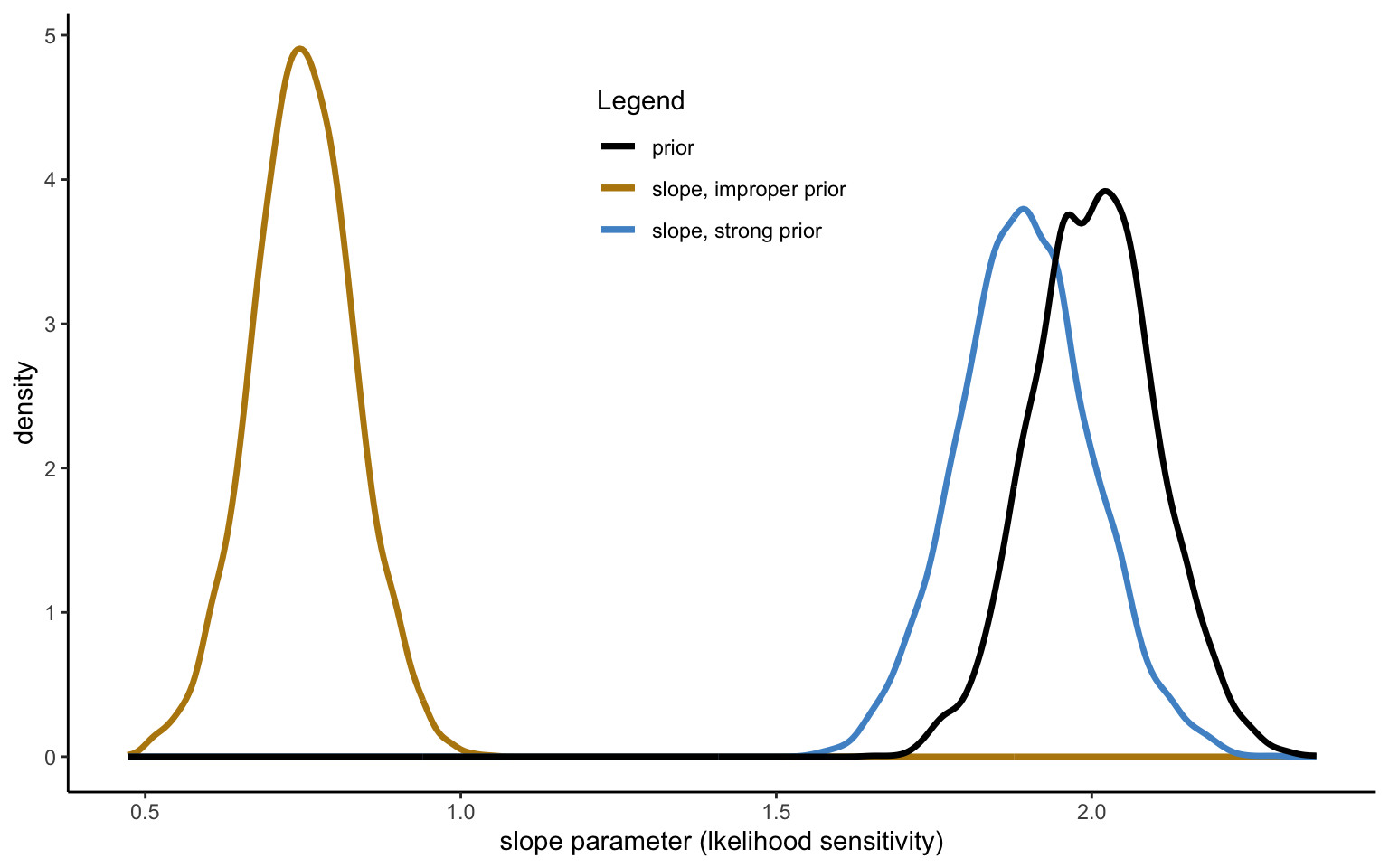
The slope parameter for this particular subject is 0.75quite typical (estimated based on a regularizing prior with mean 0.7, and a SD of 0.5). The standard error associated with the parameter, however, is quite large at 0.078, indicating that the parameter could fall anywhere between 0.59612 and 0.90188. We can see the consequence of this if we again impose the outlandish prior with mean 2 and SD 0.1. The slope is now estimated at 1.892a far cry from the original estimate. Figure 3.3 shows what is happening.
Figure 3.3: Slope parameter estimated with weak annd strong prior
3.3.5 Probit and logit regression
Let us assume that we have discrete choice data instead of a continuous variable, such as a certainty equivalent (or a present equivalent for inter-temporal choice). The main change to our setup will be that we now need to use a link function to map our model to a choice probability. Stan of course allows for the implementation of either a Probit model (using the standard normal CDF Phi or a faster approximation Phi_approx) or a Logit model. A standard logit regression will then look like this:
where we examine the choice probability as a function of the difference in expected value between the prospect and the sure amount. Let us use the data of choice under risk from Abdellaoui et al. (2011) to illustrate the estimation:
Show the R code
rd <-read_csv("data/data_rich_domain_risk.csv")rd <- rd %>%filter(low==0) %>%mutate(ev_diff = p*high - sure)# creates data to send to StanstanD <-list(N =nrow(rd), ev_diff = rd$ev_diff,choice_risky =as.integer(1- rd$choice_sure) )# compile the Stan programme:sr <-cmdstan_model("stancode/logit_ev.stan")# run the model:nm <- sr$sample(data = stanD, seed =123, chains =4,parallel_chains =4,refresh=0,init=0,show_messages =TRUE,diagnostics =c("divergences", "treedepth", "ebfmi"))print(nm, c("alpha","beta"),digits =3)saveRDS(nm,file="stanoutput/logit_ev.Rds")
In discrete choice models of decision making, the model we want to implement will typically look different from the standard model shown above. For one, we may want to look at the difference between transformed quantities, i.e. the difference between the expected utility of the wager and the utility of the sure amount. Furthermore, it is customary to add an explicit noise term to the implementation, normally reflecting a random utility setup, and which takes the form of a Fechner error in the Probit model, or of a precision term in the logistic regression. We will examine such more realistic models in due time.
3.4 Aggregate non-linear models
In this section, I will develop some nonlinear models at the aggregate level. This will go fairly quicklythere is nothing that special about these types of models. This setup will, however, lay the foundations for the more interesting models to be considered in the next chapter.
3.4.1 A simple dual-EU model
Take indifferences of the type \(c \sim (x,p)\), ie certainty equivalents for simple wagers with only one nonzero outcome. In a EU framework, we could model them as \(c^\rho = p \times x^\rho\). We know, of course, that a perfectly equivalent way of modelling them is \(c = p^\gamma \times x\), where \(\gamma \triangleq \frac{1}{\rho}\). I will work with the latter for simply because it allows for a more natural transition to the multi-parameter models we will see below. The function, in either form, could of course be easily linearized and estimated with standard regression tools (try this as an exercise), but that would miss the point of this section.
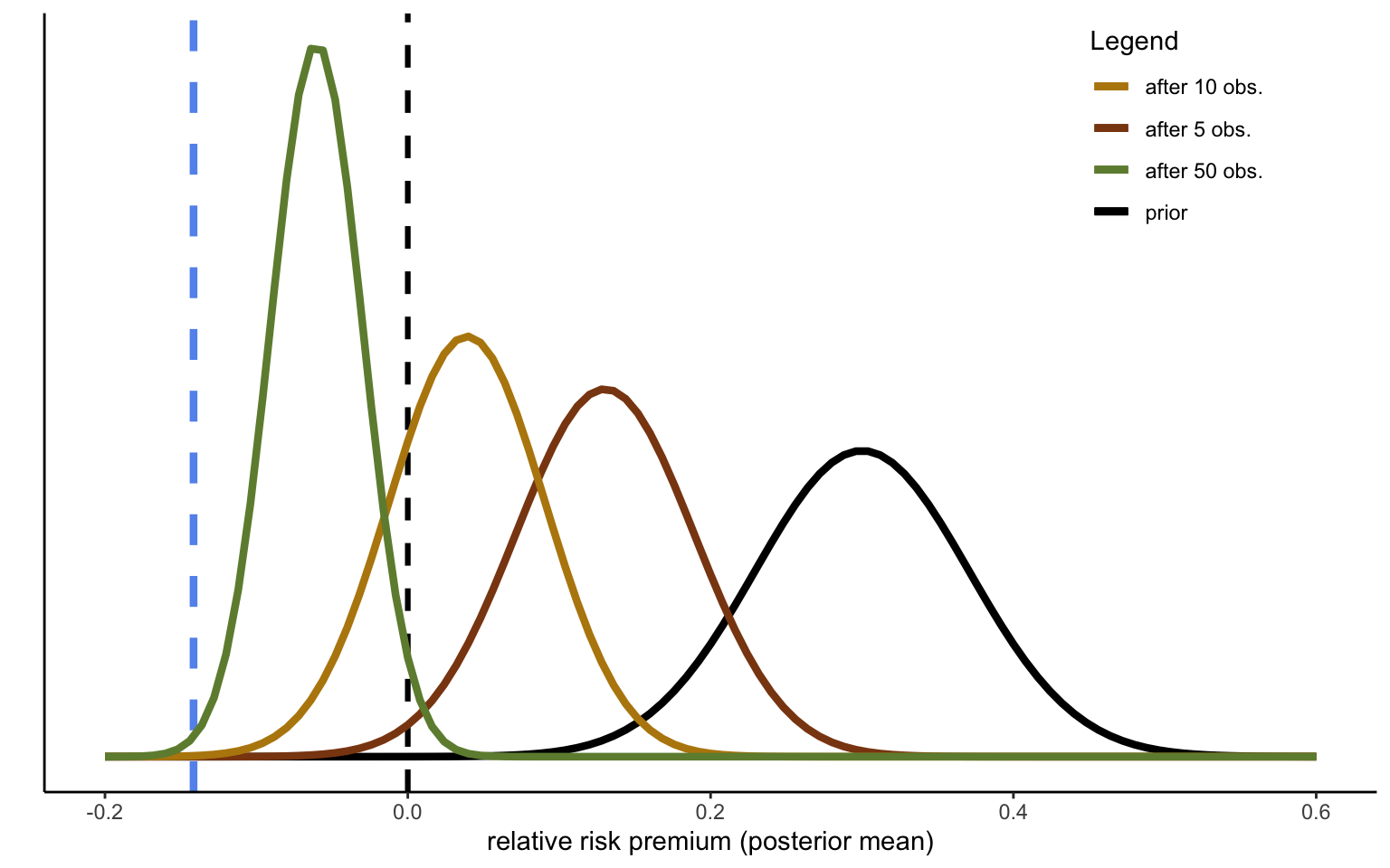
For a change, we will use the data from Vieider et al. (2018), containing CEs for some 500 subjects from rural Ethiopia. For illustrative purposes, let us first explore the data in a nonparametric way. To this purpose, let \(\pi(p)\) we a decision weight associated to the probability \(p\), so that \(c = \pi(p) x\), from which we get \(\pi(p) = \frac{c}{x}\). To keep it simple, let us restrict our attention to \(p=0.5\). We can define an index of relative risk aversion as \(rrp = p - \pi(p) = 0.5 - \pi(p)\). Risk averse subjects will have \(\pi(p)<p\), which corresponds to the typical risk aversion for moderate probabilities documented in hosts of studies. Let us enshrine this knowledge in a prior \(p(\mu) = \mathcal{N}(0.3,200^{-1})\), which I have chosen to be fairly narrow, given the large evidence base. (I am not suggesting that this is appropriate; it rather serves illustration purposes).
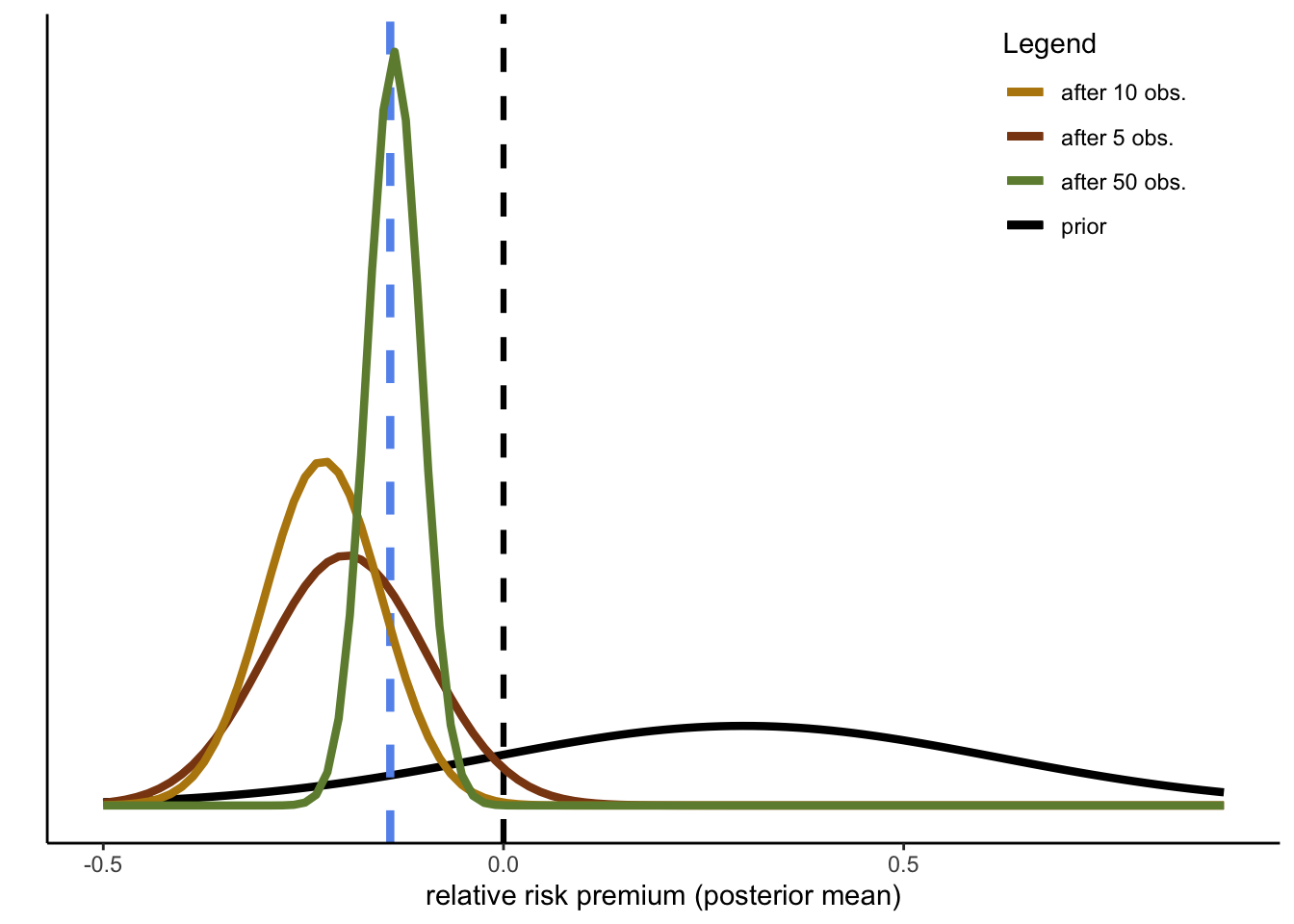
The following code is devised to extract CEs from the data. Assume now you are conducting experiments in Ethiopia for the first time. You will observe the CEs sequentially, and you can thus update your prior with one observation at a time. To keep the illustration as simple as possible, we can cheat a little and use the true sample variance from the whole dataset, so that we only have to update the mean of the prior and the connected variance using the procedures developed in the first part. Note that I will treat the data as fully exchangeable, thereby ignoring the actual data collection structure (several CEs per subject, which is solved by using only the 50-50 prospect; subjects sampled from different villages; different villages sampled from different districts (Woredas), Woredas sampled from regions). The sequential updating with 50 randomly selected observations is illustrated in Figure 3.4.
Figure 3.4: Sequential updating of decision weights
We can see that the model gradually converges to the true sample mean, indicated by the dashed blue line. How close this is to the true mean of the overall data, and how quickly the mean converges to the true mean, will of course depend on the random sample extracted (just run the simulation including the random extraction repeatedly changing the seed to convince yourself of that). One way to speed up the process is, of course, to reduce the precision of your prior. That is, if you are not convinced that everybody will necessarily decide like select samples from a handful fo WEIRD Western countries, you may choose your prior to have a wider variance, even while sticking with the same mean:
As you would expect, convergence to the true mean is both quicker and more complete.
3.4.2 Dual-EU model: Aggregate estimation
We can now proceed to aggregate estimation. I will here use all stimuli, instead of restricting attention only to 50-50 wagers as above. To this end, we can use the model below. A few comments are in order. Other than above, I have imposed mildly regularizing priors on the parameters. While it may be legitimate to impose stronger priors based on past evidence on risk aversion over much of the probability interval, there are two major counterarguments (even without taking the evidence we have seen above into account): 1) risk seeking has been found to coexist with risk aversion; 2) the novel context makes strong priors taken from other contexts questionable.
Another change from the models seen to far is that I now define several auxiliarity variables in the model block (which are thus available only locally), which I then enter into subsequent computations. This is arguably not necessary in a simple model such as this one, but it will become essential as the model complexity increases. Also, I am using a loop instead of vectorizing, because a vector taken to a power is not defined (NOTE: The Stan development team has been working on a function allowing to take powers of individual vector elements, which would overcome this issue).
Show the R code
data{int<lower=1> N;array[N] real ce;array[N] real high;array[N] real p;}parameters{real<lower=0> gamma;real<lower=0> sigma;}model{//auxiliary variables (available locally in model block):vector[N] wp;vector[N] pv;// diffuse priors: sigma ~ normal( 0.2 , 0.5 ); gamma ~ normal( 1 , 0.5 );//model: for ( i in1:N ) { wp[i] = p[i]^gamma ; pv[i] = wp[i] * high[i]; ce[i] ~ normal( pv[i] , sigma * high[i] ); }}
We are now ready to estimate the model:
Show the R code
eth <-read.csv("data/data_ETH.csv")# creates data to send to StanstanD <-list(N =nrow(eth), ce = eth$equivalent,high = eth$high,p = eth$probability)# compile the Stan programme:sr <-cmdstan_model("stancode/agg_DEU.stan")# run the model:nm <- sr$sample(data = stanD, seed =123, chains =4,parallel_chains =4,refresh=0,init=0,show_messages =TRUE,diagnostics =c("divergences", "treedepth", "ebfmi"))nm$print(c("gamma", "sigma"), digits =3,"mean", SE ="sd", "rhat" ,~quantile(., probs =c(0.025, 0.975))) nm$save_object(file="stanoutput/agg_DEU_ETH.Rds")
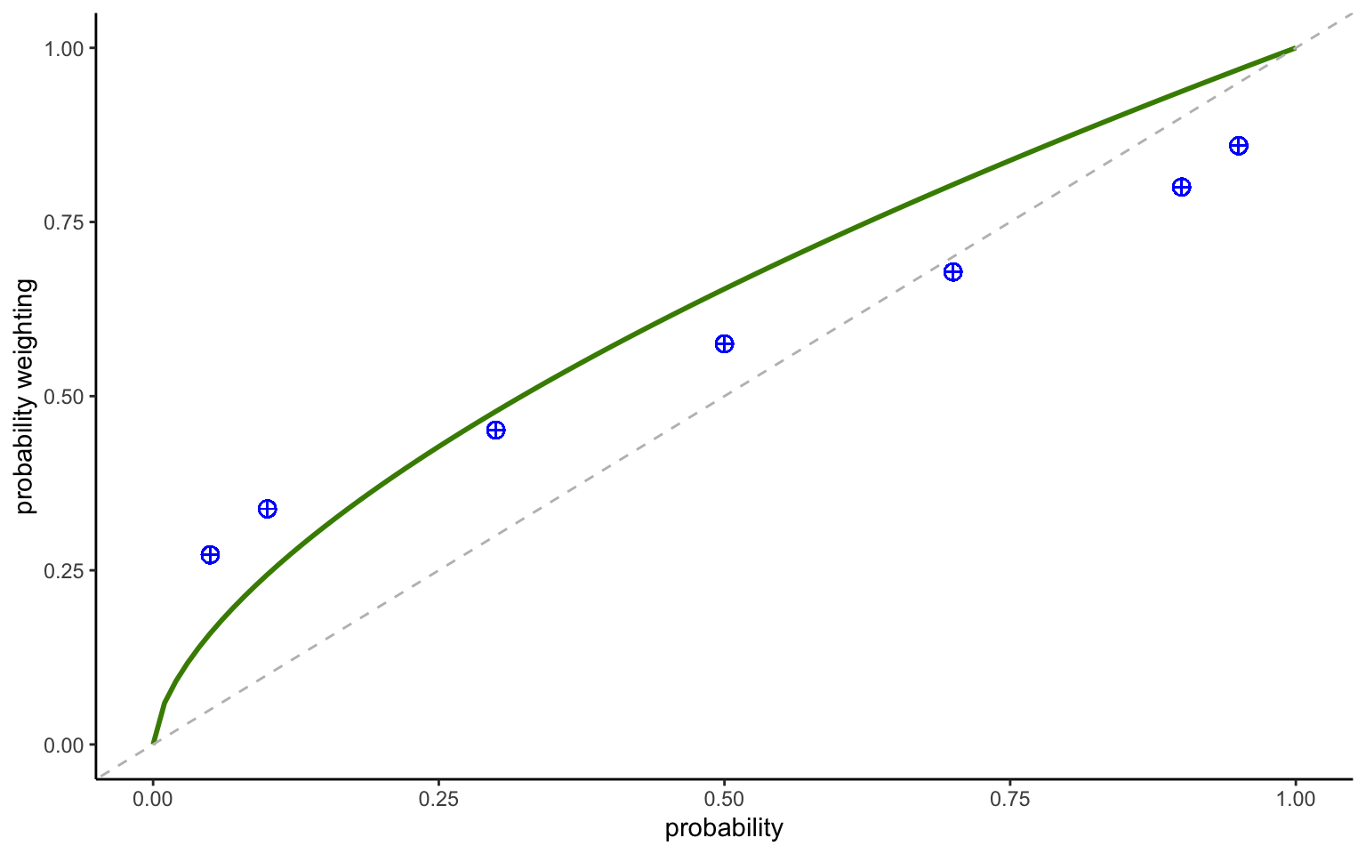
We can now compare the fitted data to the nonparametric data points to check the validity of our model. This is straightforward in a dual-EU setting, where the nonparametric decision weights are simply \(\frac{c}{x}\). A rigorous analysis might add confidence intervals around the fitted function. This is usually done with simulations. Bayesian analysis is particularly convenient here, since we can simply sample from the posterior. Creating a graph including the uncertainty intervals is left for an exercise.
Show the R code
deu <-readRDS("stanoutput/agg_DEU_ETH.Rds")de <-as_draws_df(deu)m <-mean(de$gamma)eth <- eth %>%mutate(dw = equivalent/high) %>%group_by(probability) %>%mutate(mean_dw =mean(dw)) %>%ungroup()pw <-function(x) (x^m)ggplot(data=eth, aes(x=probability,y=mean_dw)) +stat_function(fun = pw,color="chartreuse4",size=1) +xlim(0,1) +geom_point(size=3, color="blue",shape=10) +geom_abline(intercept=0, slope=1,linetype="dashed",color="gray") +labs(x ="probability", y ="probability weighting")
Figure 3.5: Dual-EU model with power weighting function
The aggregate data shown in Figure 3.5 indicate a concave pattern, whereas risk aversion requires a convex pattern. After looking at the nonparametric data patterns above, this is no surprise. Clearly, the model might benefit from a second parameter, allowing it to capture the coexistence of risk seeing and risk aversion for different probability levels (or simply a different functional form, achieving the same with just one parameter).
3.4.3 Multiple parameters
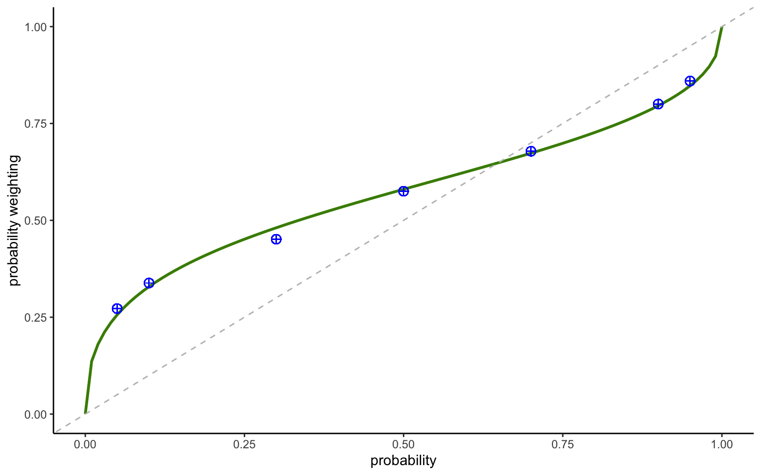
There is nothing special about having a model with more than one parameter (technically, the model above already had two including the variance). The following code implements a (nonlinear version of the) Goldstein-Einhorn weighting function:
eth <-read_csv("data/data_ETH.csv")# creates data to send to StanstanD <-list(N =nrow(eth), ce = eth$equivalent,high = eth$high,p = eth$probability)# compile the Stan programme:sr <-cmdstan_model("stancode/agg_DEU_GE.stan")# run the model:nm <- sr$sample(data = stanD, seed =123, chains =4,parallel_chains =4,refresh=0,init=0,show_messages =TRUE,diagnostics =c("divergences", "treedepth", "ebfmi"))nm$print(c("delta","gamma", "sigma"), digits =3,"mean", SE ="sd", "rhat" ,~quantile(., probs =c(0.025, 0.975))) nm$save_object(file="stanoutput/agg_DEU_GE.Rds")
Figure 3.6: Dual-EU model with power weighting function
We can now compare the fitted function to the nonparametric data points to check the validity of our model. This is shown in Figure 3.6. The fit to the aggregate data is no almost perfect.
3.4.4 A discrete choice DU model
To illustrate the estimation of a multiparameter model in a discrete choice setup, I will use some discreet choice data of tradeoffs between sooner-smaller against larger-later options obtainned in an incentivized classroom experiment. Before launching into the estimations, however, it is always useful to obtain an idea of the main patterns present in the data using nonparametric methods. This can then serve as a check for the patterns one observes in the structural model, and it is here left for an exercise.
The data consist of a large number of binary choices between a smaller-sooner amount and a larger later amount, which is kept fixed at 50 Euros. Say we are interested in quasi-hyperbolic discounting, i.e. in whether the choice patterns exhibit present-bias. This can be captured by the discounting function \(D(t) = \beta \times exp(-rt)\), where \(\beta<1\) indicates present-bias. For \(t=0\), the function will be \(D(0) = 1\). When both outcomes are pushed to the future, \(\beta\) drops out of the model and discounting reduces to an exponential model. (In practice, present bias will be confounded by subadditivity in the data, which the function cannot handle; however, I am interested in the technicalities of the estimation process, rather than in the accuracy of the inferences drawn).
We can also use this example to illustrate another Bayesian featureso-called regions of practical equivalence, or acceptance regions. These correspond to parameter intervals for which we will accept the null hypothesis. Other than in frequentist statistics, which invariably tests point hypotheses, Bayesian statistics allows both for rejecting and for accepting the null hypothesis. Let us assume an acceptance region of \(>0.97\) (of of \(>0.97\) and \(<1.03\), if we think there might be a chance of finding the opposite of present bias).
Now we are ready to run the structural model. Other than in the simple regressions seen above, we will want to add an explicit error term. Let the discounted utility of the smaller-sooner option be \(D(s)y\), with the discounted utility of the larger-later option described by \(D(\ell)x\). The discount function \(D(s)\) will be the exponential function, except when the sooner time is 0, in which case there will be a \(\beta\) in \(D(\ell)\) to account for present bias. We can then implement a logistic model by means of the following link function, capturing the probability with which the larger-later option is chosen: \[
Pr[(x,\ell) \succ (y,s)] = \frac{e^{\lambda D(\ell)x}}{e^{\lambda D(\ell)x} + e^{\lambda D(s) y}},
\] where \(\lambda\) is a inverse temperature parameter, so that \(\lambda = \infty\) corresponds to a noiseless process. We can code the model as follows:
Show the R code
data{int<lower=1> N;array[N] int id;array[N] real x;array[N] real y;array[N] real s;array[N] real l;array[N] int cl;array[N] int s0;}parameters{real<lower=0> rho;real<lower=0> beta;real<lower=0> lambda;}model{vector[N] dus;vector[N] dul;vector[N] prl; rho ~ normal(0.1, 0.2); beta ~ normal(1, 0.5); lambda ~ normal(10, 20);for ( i in1:N ) { dus[i] = exp(-rho * l[i] ) * y[i]; dul[i] = beta^s0[i] * exp(-rho * l[i] ) * x[i]; prl[i] = exp(lambda * dul[i])/( exp(lambda * dul[i]) + exp(lambda * dus[i]) ); cl[i] ~ bernoulli( prl[i] ); }}
Show the R code
d <-read_csv("data/data_NCT.csv")da <- d %>%mutate(immediate =ifelse(ts==0 , 1 , 0)) %>%filter( progress==100)#create data to send to StanstanD <-list(N =nrow(da), id = da$id,x =abs(da$large),y =abs(da$small),s = da$ts,l = da$tl,cl = da$choice_later,s0 = da$immediate)# compile the Stan programme:sr <-cmdstan_model("stancode/agg_QH_logit.stan")# run the model:nm <- sr$sample(data = stanD, seed =123, chains =4,parallel_chains =4,refresh=200,init=0,show_messages =TRUE,diagnostics =c("divergences", "treedepth", "ebfmi"))nm$print(c("rho","beta", "lambda"), digits =3,"mean", SE ="sd", "rhat" ,~quantile(., probs =c(0.025, 0.975)))nm$save_object(file="stanoutput/agg_qh_logit.Rds")
We find substantial present bias. It is clear from the distribution of the parameter that iit falls very far from the region of accepance, so that we can reject the null hypothesis.
While we have coded the inverse-logit link function by hand using the ratio of exponentials. Aas a rule, this is not needed in Stan, which offers (more efficient) pre-rpogrammed funcion. n particular, the bernulli_logit function reunites the link function and Bernouli ransformation in one neat function. Here, I will illustrate how to code a Probit model using Stan’s pre-existing functions.
Show the R code
data{int<lower=1> Narray[N] int id;array[N] real x;array[N] real y;array[N] real s;array[N] real l;array[N] int cl;array[N] int s0;}parameters{real<lower=0> rho;real<lower=0> beta;real<lower=0> sigma;}model{vector[N] disc;vector[N] udiff; rho ~ normal(0.1, 0.2); beta ~ normal(1, 0.5); sigma ~ normal(0.2, 0.5);for ( i in1:N ) { dus[i] = exp(-rho * l[i] ) * y[i]; dul[i] = beta^s0[i] * exp(-rho * l[i] ) * x[i]; udiff[i] = (dul[i] - dus[i])/(sqrt(2) * sigma); cl[i] ~ bernoulli( Phi( udiff[i] ) ); }}
Show the R code
d <-read_csv("data/data_NCT.csv")da <- d %>%mutate(immediate =ifelse(ts==0 , 1 , 0)) %>%filter( progress==100)#create data to send to StanstanD <-list(N =nrow(da), id = da$id,x =abs(da$large),y =abs(da$small),s = da$ts,l = da$tl,cl = da$choice_later,s0 = da$immediate)# compile the Stan programme:sr <-cmdstan_model("stancode/agg_QH.stan")# run the model:nm <- sr$sample(data = stanD, seed =123, chains =4,parallel_chains =4,refresh=200,init=0,show_messages =TRUE,diagnostics =c("divergences", "treedepth", "ebfmi"))nm$print(c("rho","beta", "sigma"), digits =3,"mean", SE ="sd", "rhat" ,~quantile(., probs =c(0.025, 0.975)))nm$save_object(file="stanoutput/agg_qh.Rds")
The quasi-hyperbolicity parameter we obtain is virtually identical to the one we obtained from the logistic model above. The discount rate, however, is slightly larger. That is of course not surprising, given that we have estimated a different model. Statisticallly speaking, however, the two discount rates aare not clearly distinguishable, showcasing the similarity between the two models.
3.5 Individual-level estimation
While we have so far focused on aggregate estimations, it is often of interest to present individual-level estimations. There is double good news in this respect. Not only can the aggregate-level techniques we have just seen be applied to individual-level estimations, but they are typically also both easier to obtain and more stable than using maximum likelihood techniques. This section starts by illustrating some of the problems in traditional ML estimation of individual-level estimations, and how to overcome them in Bayesian estimations.
3.5.1 The trouble with individual-level estimates
Individual-level estimations tend to be quite delicate due to the reduced number of data points that are typically available. Overfitting sparse noisy data thus becomes a major concern. This is particularly true in multi-parameter models such as prospect theory, where multiple unconstrained parameters compete to pick up similar behavioural motives. In the presence of noise, the different dimensions may not be well separated, giving rise to likelihoods with local maxima, or to flat regions presenting similar likelihoods. It is thus doubly important to check the results against the data. Estimates may be sensitive to starting values of the parameters when data are noisy, which constitutes itself a type of identifiability problem. The standard solution in ML estimation is to run repeated estimations for each individual using different starting values (a so-called grid search procedure), which serves to detect whether the estimations may converge to different maxima of the likelihood function, some of which may be local. The Bayesian routines we use here do this automatically to some extent, if every chain is started at randomly generated values (which is done automatically if no initial values are specfied). It is thus important to check whether the chains “mix” properly, i.e. the different chains should explore the same parameter values.
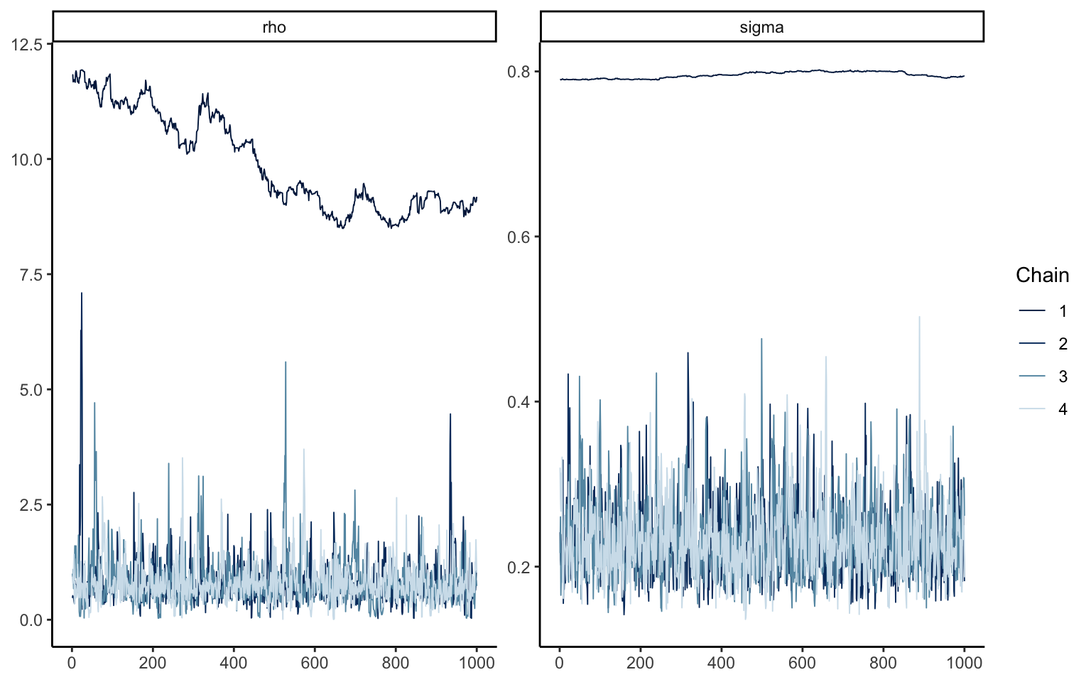
We illustrate this issue by estimating the individual-level parameters of subject 65 in the Zurich 2006 data of Bruhin, Fehr-Duda, and Epper (2010) using the aggregate routine used previously, which imposes improper priors and is thus equivalent to a ML estimator, i.e. an “emprical Bayes” estimation (the data are not included inn the repository, but can be downloaded from https://www.econometricsociety.org/publications/econometrica/2010/07/01/risk-and-rationality-uncovering-heterogeneity-probability/supp/7139_data%20and%20programs_0.zip). The diagnostic summary indicates that, while three chains had no problems, chain 4 had a fairly large share of so-called “divergent iterations” (as indicated by the warning: Warning: 362 of 4000 (9.0%) transitions ended with a divergence; NOTE: the exact value may differ depending on the seed you set and the resulting random starting values). While such divergent iterations may at times occur in nonlinear estimation, they should always be checked to be sure that they do not signal fundamental problems with the estimation (and 9% is a lot, raising all kinds of red flags).
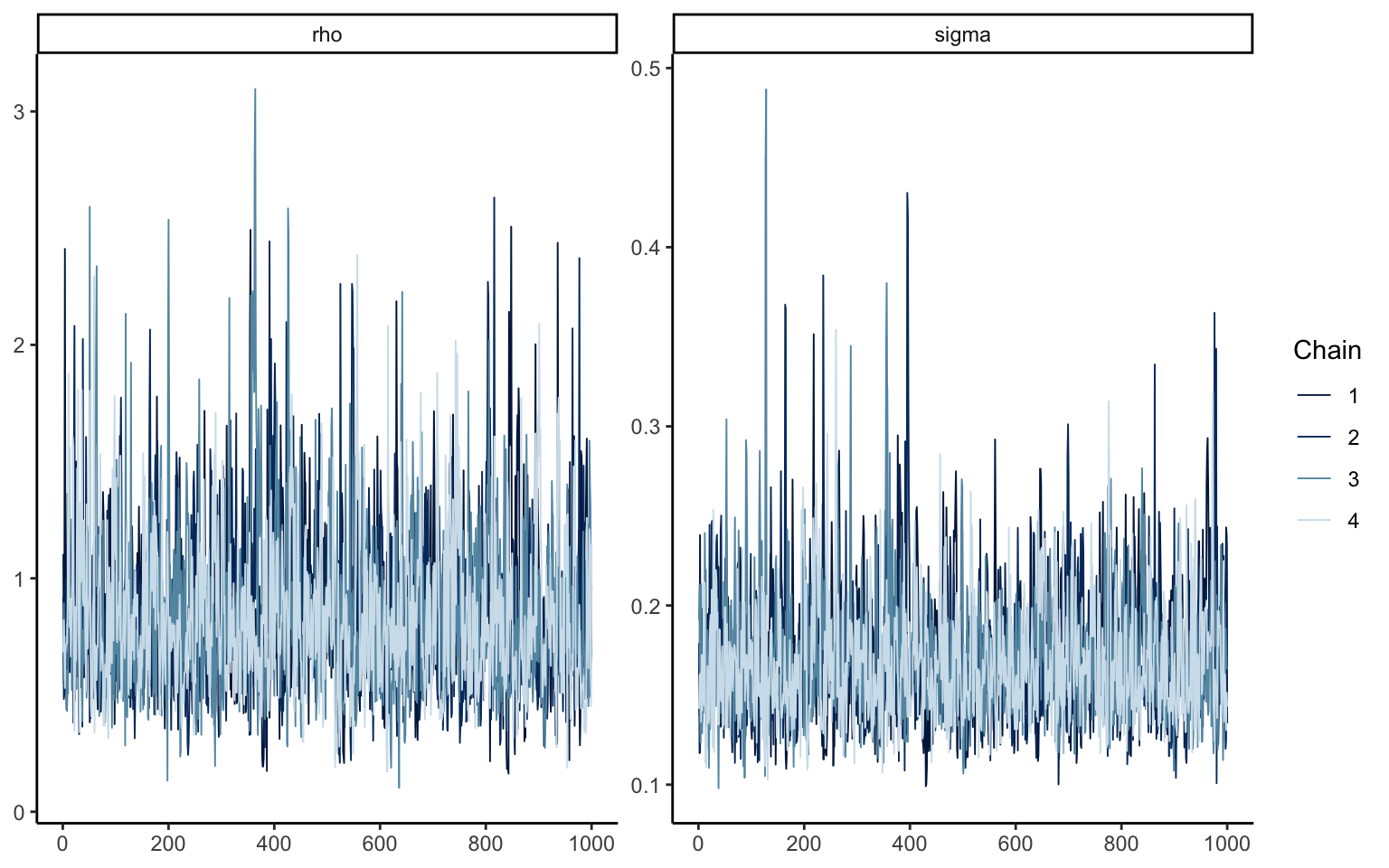
p65 <- s65$draws(format ="array")mcmc_trace(p65, pars =c("rho", "sigma"))
Figure 3.7: Trace plot for subject 65, Emprical Bayes estimation
Figure 3.7 shows the trace plot, i.e. the parameter points visited by the simulation algorithm in each chain, for parameters \(\rho\) and \(\sigma\). Three chains can be seen to have mixed properly (although some extreme spikes are indicative of large posterior uncertainty). One chain, however, produces very different values for both parameters, as well as displaying high degrees of autocorrelation. We should thus not accept the estimates, since these patterns indicate major problems in the estimation.
The results just seen clearly indicate trouble in the estimation routine. Notice that, by choosing appropriate starting values by hand, and possibly even with a given seed, you may be able to sweep these issues under the rug. That would, however, be a terrible idea. What these results indicate is very simply that the estimates we obtained cannot be trusted. It is thus not enough to simply force the divergent chain towards the others by brute force, and we will need to come up with an alternative procedure. Luckily, that is easily done.
3.5.2 How to overcome issues in individual estimates
One way of overcoming this issue is to impose so-called regularizing priors. Such priors are typically determined to be both noninformative and diffuse. Below, we reproduce a code snippet of the model block, where priors are now given for the 4 model parameters. Note that the mean of the prior is fixed at 1, which for the model parameters \(\rho\), \(\gamma\), and \(\delta\) coincide with the values entailing expected value maximization. This is the sense in which the values are noninformative, since we do not actually incorporate any prior knowledge, e.g. on the near-universality of likelihood-insensitivity (see below). Furthermore, by choosing a standard deviation that is suitably large, we make sure that the data can easily overpower the prior. In the case illustrated below, 95% of the probability mass in the prior is attributed to parameter values ranging between \([-1,3]\) (even though we cut off the distribution at 0, since values below 0 are not admissible for most of the parameters). This gives a large enough berth to accommodate any plausible parameter values. Even though this prior does not restrict the estimations in any substantive way, it may nevertheless be sufficient to point the algorithm in the right direction, thus avoiding the issues described above.
Below, I repeat the estimation for subject 65 with the non-informative, diffuse priors described above. The divergent iterations disappear, and the chains now appear to mix properly, as can be seen from Figure 3.8. This shows the power of priors. Even though the priors do not restrain the parameter estimates in any substantive way, such mildly regularizing priors are sufficient to discipline the estimates and avoid convergence problems in this case. Note, however, that in general one ought to be careful when choosing priors for sparse data, as we have done here. Imposing specific values and making the priors too narrow may well sway the estimate. It is thus always necessary to check the fit to the data in addition to executing convergence checks, such as illustrated above. It is also a good idea to vary the prior and to make sure that the particular results obtained are not sensitive to different priors falling in a reasonable range.
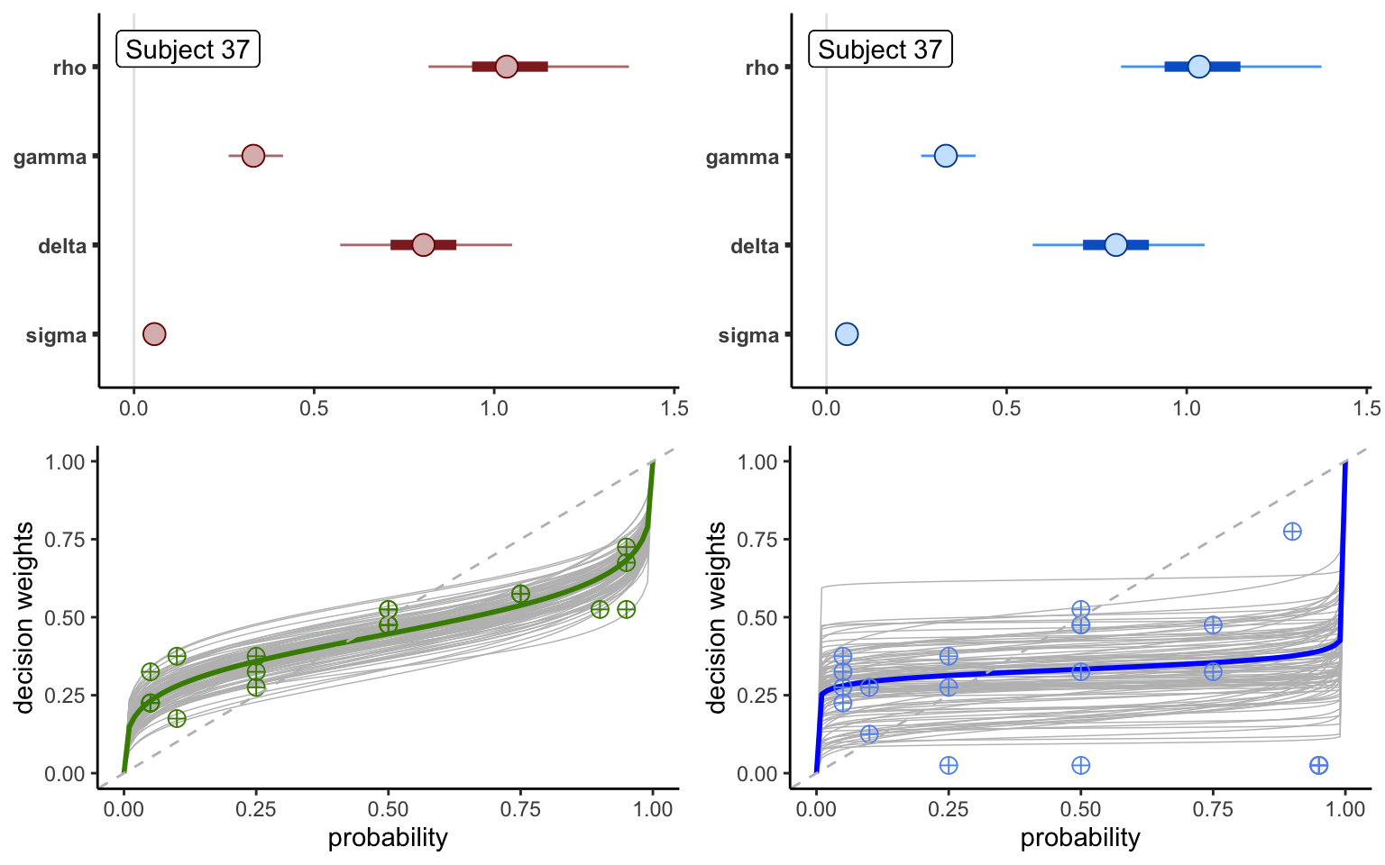
Figure 3.9: Parameters and functions for subjects 37 and 65
Figure 3.9 shows the parameter estimates for two individuals (top panels): the already-discussed subject 65, and subject 27 from the same dataset, jointly with the posterior uncertainty intervals. The estimated parameter values are fairly similar, although subject 65 displays lower likelihood-sensitivity. In addition, subject 65 has larger noise levels, as reflected by larger values of the noise standard deviation \(\sigma\). Notice furthermore that this larger noise level is not only reflected in the larger value of \(\sigma\), but also seeps through to all the other parameters, which are estimated with less precision (that is, they have larger uncertainty intervals). This is particularly evident for the utility curvature parameter \(\rho\) and the optimism parameter \(\delta\). This is indeed a common problem in PT estimations, since optimism and utility curvature capture similar motives, and can be difficult to tease apart in noisy data.
The bottom panels of Figure 3.9 plot the fit of the probability weighting functions to the nonparameteric data points for the same two subjects. The thin lighter lines constitute randomly selected draws from the Bayesian posterior, and represent the overall uncertainty surrounding the mean estimate of the probability weighting function. The draws for subject 37 stay relatively close to the mean estimate, but are still dispersed enough to encompass almost all the nonparametric data points. The lines surrounding the mean estimate for subject 65, however, are very dispersed. This indicates a very low degree of confidence in the mean parameters, and is a symptom of the uncertainty attached to the single parameters, as already discussed above. The fact that these lines move up or down while staying almost parallel is an indication that the uncertainty affects mostly the optimism parameter \(\delta\), whereas likelihood-sensitivity \(\gamma\) is estimated with a much higher degree of confidence.
3.5.3 Batch estimation of individual parameters
One possibility to obtain individual-level data is to use the aggregate model from above, and to apply it individual-by-individual in a loop. That approach, however, is rather tedious. Here, we will take a different approach. We will carefully leverage priors to nudge individual-level estimations in the right direction, as illustrated above in the individual-level estimations. In addition, we will use a Stan model that yields fixed-effects estimates of all individual-level parameters in one go.
Below, we show the code of the Stan programme. The main trick is that we now estimate parameter vectors, the elements of which represent estimates of different subjects. Note that the identifier needs to start at 1 and comprise consecutive numbers for the code to work. If this is not the case, odd results may appear due to inconsistent mapping between IDs and parameter vectors (typically, the code will attempt to obtain estimates for a number of individuals equal to the maximum ID, with the values for missing individuals sampled from the priors). The priors as usual nudge the estimation into a region where we would expect the parameters to lie, without imposing any strong prior knowledge. [NOTE: here, as above, we limit \(\rho\) at 0 from below; a more general procedure would be to write conditional statements whereby \(u(x) = x^\rho\) if \(\rho > 0\), \(u(x) = ln(x)\) if \(\rho \equiv 0\), and \(u(x) = -x^\rho\) if \(\rho < 0\)].
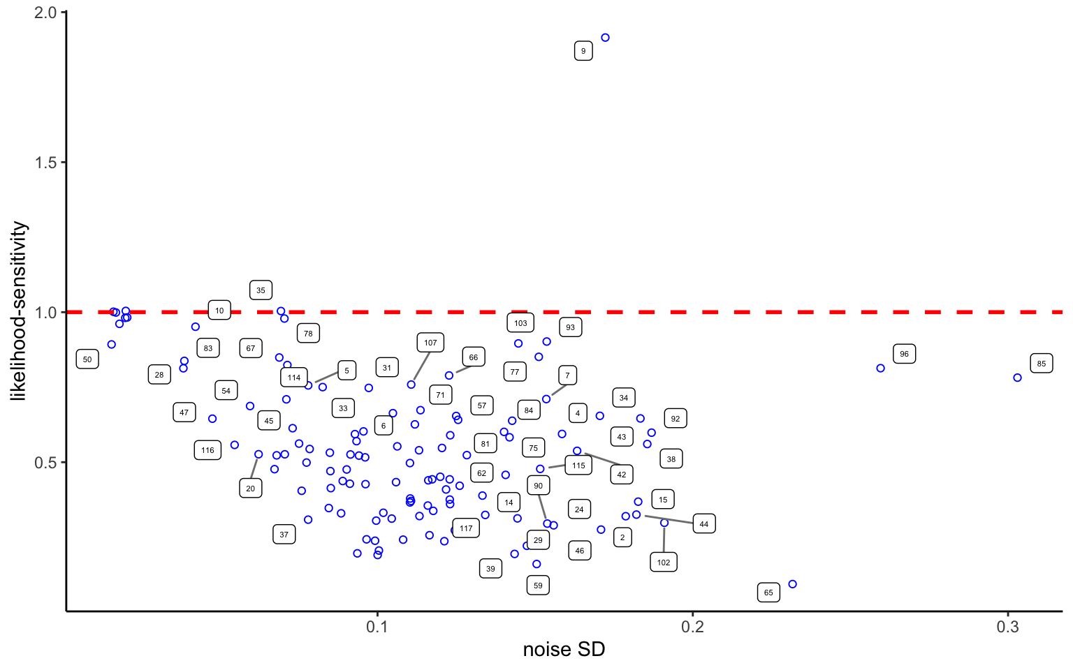
Figure 3.10: Scatter plot of noise annd likelihood-sennsitivity, fixed effects
Figure 3.10 shows a scatter plot of the noise SD against likelihood-sensitivity in the individual-level fixed effects estimates. Some patterns stand out in the data. A handful of individuals have sensitivity arbitrarily close to 1, combined with very low noise levels. These are the expected value maximizers described in the mixture model of Bruhin, Fehr-Duda, and Epper (2010). Overall, likelihood-sensitivity and noise appear to show a negative correlation. That being said, individuals 37 and 65, for whom we have examined the individual patterns above, both show low levels of likelihood-sensitivity, yet have very different levels of noise. We will re-examine some of these patterns shortly, in the context of hierarchical estimation. For now, note also subject 9—a subject with fairly large noise, and the only subject displaying likelihood-oversensitivity. There is no reasonn to think that the estimatte has not converged properly. Nevertheless, we should be careful before accepting such a large outlier (and possibly enntering this parameter into a regression). We will dscuss how to deal with this inn a principled way in the next chapter.
3.5.4 Regression of parameters
It may be tempting to build parameter regressions directly into an aggregate model. While technically possible, this would ignore that fact that we have a multiplicity of observations for each individual, and would thus yield biased results. We can, however, easily estimate a regression using individual-level parameters such as mentioned above. A very simple approach would be to obtain the individual-level estimates, and then to use the means of the parameter estimates (or the medians for that matter) in a second-stage regression. The main problem with this sort of approach is that we ignore uncertainty surrounding the parameters. There are two ways around this. We can either estimate the regression in the same model estimating the parameters themselves, thus taking a long the entire posterior uncertainty about the parameters; or we can build an measurement error model that makes use of the second-order information summarizing the distribution of the parameters around their mean.
We will again use the Zurich 2006 data used above. The main model will be identical to the one used above. Assume now we want to regress only likelihood-senstivity \(\gamma\) on some background characteristics—say the gender and high income status of the subject. The trick will be to add a second loop after the first one. This loop is now defined at the level of the individual, thus eliminating the dimentionality problem mentioned above. Running the regression within the same model further ensures that all the parameter uncertainty is taken into account in the estimation. Note also that we need to define the design matrix at the level of the inndividual, so that we will first need to obtain data with only one observation per subject to create that matrix.
fe <-readRDS("stanoutput/ind_ZCH06_fixed_reg.RDS")fe$print(c("beta", "tau"), digits =3,"mean", SE ="sd", "rhat" ,~quantile(., probs =c(0.025, 0.975)))
 variable   mean    SE  rhat   2.5%  97.5%
  beta[1]  0.538 0.029 1.000  0.483  0.595
  beta[2] -0.098 0.040 1.001 -0.177 -0.017
  beta[3]  0.055 0.107 1.001 -0.149  0.268
  tau      0.158 0.017 0.999  0.127  0.194
The regression results show that women have lower likelihood-sensitvity thann men. There is no clear effect of high income status (which is not surprising if you look at he data—there are only very few subjects for which the dummy takes the value 1).
In general, you will typically run the regression for all parameters at once. One way of doing this is using an equation for each parameter inside the loop. A more efficient way of coding this may be to collect the parameters into a vector, and to estimate a matrix of parameters. This is left as an exercise. Let me conclude this discussion by noting that the code used here is very flexible. For instance, you could just as well use the parameters on the right-hand side of the equation. We will return to regression analysis when discussing hierarchical models in the next chapter.
3.5.5 Should one do individual-level estimation?
When estimating a data set like this, should one pool the data, implicitly assuming that all the choices come from one single agent? Or should one recur to individual-level estimations, thus treating every individual as completely distinct? A principled way of going about this question could be to compare within-individual variation in responses to between-individual variation. If between-individual variation is small relative to within-individual variation, then one could pool the data; if between-individual variation is large relative to within-individual variation, then one could estimate the parameters subject-by-subject. However, why not do both at once and let the endogenously-estimated variance components decide how much weight to put on individual versus aggregate estimates?
Exactly this is achieved in (Bayesian) hierarchical models. The model endogenously estimates between-subject variation, as well as within-subject variation for each subject. Individual-level parameters are then “shrunk” toward the aggregate mean in function of their noisiness (more noisy data are shrunk more) and of their distance to the aggregate mean (outliers are shrunk more than data close to the mean). Such models can indeed be shown to maximize out-of-sample predictive power by discounting noisy outliers. Alas, hierarchical models are typically still only mentioned in passing in econometrics textbooks aimed at economists. They do, however, constitute the workhorse statistical tool in other disciplines, such as educational sciences, psychology, epidemiology, and medicine. Although hierarchical models can be estimated by maximum likelihood routines using so-called empirical Bayes algorithms, they are inherently Bayesian. The aggregate-level estimate indeed serves as an endogenously-estimated prior for lower-level estimates. Economists ignore such models at their own risk, since neglecting hierarchical structure where it exists can lead to severe bias in the estimation results.
3.6 Stan workflow
It is important to build up a proper workflow in Stan. This involves many aspects. Two I would like to stress are gradual model building, and simulations.
The models we have seen thus far are exceedingly simple and do not need much particular attention. As we move to more complex (and more interesting!) models, however, it will be important to carefully build up the models step by step. The general recommendation is to build up the models gradually, starting from simpler models, and then only gradually adding additional parameters and more structure. This avoids thorny issues with models not converging for no apparent reason, or parameters that are not identified (this can be difficult to spot in Stan, since a completely unidentified parameter may simply converge to its prior; i.e. the parameter will be `simulated’ rather than being estimated, which can be easy to miss if priors are informative).
Another important topic is model convergence. This is covered in the manual and in many blog posts, and I will not disscuss this in depth. In general, hints of problems are 1) large R_hat values (usually, anything above 1.05 should be considered as suspicious, and values above 1.1 should ring alarm bells); and especially 2) divergent iterations (these manifest in warnings post-estimation). While some divergent iterations will often occur in complex and high-dimensional non-linear problems, as a general rule these should always trigger a convergence check. Finally, low numbers of effective samples are also problematic and often indicate difficulties of the algorithm exploring the parameter space. Reparametrization of the model is often the solution (we will see some examples later; also consult the manual).
Stan uses a default of 1000 warmup iterations and 1000 samples per chain, and this will be plenty for most purposes if the model is well-specified. If the model is not efficient, just cranking up the samples will be of limited use. An exception when you may want to increase the number of samples is when examining a precise hypothesis concerning the tails of the distribution (e.g., whether the evidence in favour of a hypothesis is more or less than 95%). In cases that fall close to that value, this may well make a difference, since for typical distributions such as the normal there will be relatively few observations in the tails. In general, such precise cutoffs are not very relevant from a Bayesian point of view, but we all know that the average referee may well have a different take of this issue.
Simulations are an important part of the Stan workflow. An interesting feature in Stan is that it allows you to use the Stan code itself to generate simulations. In particular, data are then simulated starting from the priors you have specified, so that you may want to specify informative priors. Note, however, that simulating data from Stan does not necessarily replace traditional simulation in R. Simulations directly from Stan can be useful to check your model. However, recoverability of parameters is best tested using simulations from R, since writing two independent codes to simulate and recover the parameters reduces the likelihood of mistakes.
Abdellaoui, Mohammed, Aurélien Baillon, Lætitia Placido, and Peter P. Wakker. 2011. “The RichDomain of Uncertainty: SourceFunctions and TheirExperimentalImplementation.”American Economic Review 101: 695–723.
Bouchouicha, Ranoua, and Ferdinand M. Vieider. 2017. “Accommodating Stake Effects Under Prospect Theory.”Journal of Risk and Uncertainty 55 (1): 1–28.
Bruhin, Adrian, Helga Fehr-Duda, and Thomas Epper. 2010. “Risk and Rationality: UncoveringHeterogeneity in ProbabilityDistortion.”Econometrica 78 (4): 1375–1412.
Kruschke, John K. 2013. “Bayesian Estimation Supersedes the t-Test.”Journal of Experimental Psychology: General 142 (2): 573.
Vieider, Ferdinand M., Abebe Beyene, Randall A. Bluffstone, Sahan Dissanayake, Zenebe Gebreegziabher, Peter Martinsson, and Alemu Mekonnen. 2018. “Measuring Risk Preferences in Rural Ethiopia.”Economic Development and Cultural Change 66 (3): 417–46.