Show the R code
data{
int<lower=0> N;
vector[N] ce;
vector[N] p;
}
parameters{
real alpha;
real beta;
real<lower=0> sigma;
}
model{
ce ~ normal(alpha + beta * p , sigma) ;
}Hierarchical models are seldom discussed in much detail in econometrics textbooks used in economics. They are, however, essential tools in epidemiology, psychology, and education research. A large part of the reason for that is historical and down to path dependence. In panel data analysis, dummies at the lowest level of analysis have long been used to implement “fixed effects”, thus allowing for clean identification and avoiding that estimated effects be contaminated by selection effects. This is an important goal, albeit one that can be easily obtained using alternative implementations providing more flexibility.
Hierarchies are extremely common. And while ignoring such hierarchies where they are relevant may result in biased estimators, imposing hierarchical structure where it is not relevant is (almost) costless: the estimator will simply collapse to its OLS equivalent. Economists thus ignore hierarchies at their own risk. Below, I will give a number of examples of cases that are best thought of as hierarchies. Classical cases are, for instance, measurement error models or meta-analysis, or stratified experimental or survey designs. Far from being a marginal or specialist topic, hierarchical modelling can be used to tackle a large variety of practical problems, such as for instance concerns about multiple testing that are often voiced in classical statistics.
Interestingly, the opposite concern of insufficient power in single studies can be addressed by exactly the same means, showing how both share a common origin (see discussion of the canonical 8 schools example). We will also see how hierarchical analysis is essential when trying to capture a complex sampling setup. I will provide an extended example based on panel data analysis. I will also show how stratified sampling setups ought to be reflected in the data analysis, and how explicitly modelling the data collection procedures can actually affect our conclusions (or rather, how ignoring such structure may lead to loss of information and biased inferences).
To see the value of hierarchical modelling in nonlinear estimation, imagine the following situation. You have collected choice data from a large set of individuals, each of whom has made a number of choices e.g. between lotteries. How should you analyze these data? Obvious responses that have been given to this question in the literature are: 1) we can assume that all choices come from a representative agent, and run an aggregate estimation; or 2) We treat each subject as a separate unit, and estimate the model for each of these units. We have seen both approaches in the last chapter. The problem is that aggregate estimation may ignore heterogeneity between agents, and individual-level estimation runs the risk of overfitting sparse noisy data.
A more principled approach may thus be to first assess the variance in responses for each agent, possibly after conditioning on a model (i.e., obtain the residual variance after fitting a given model). This corresponds to an individual-level estimate. Then compare the within subject variation to the variation in parameters across subjects. Little variation across subjects may then indicate the legitimacy of aggregate estimation, or vice versa. However, why not let the relative variances determine which weight each observation gets? That is exactly what hierarchical analysis does. It thus constitutes a principled way of compromising between aggregate and individual data patterns, which are taken into account in a way that is proportional to their relative precision (the inverse of the variance).
Yet a different intuition can be had if we think of the aggregate estimation as the prior. We have discussed in the previous chapter that defining a prior can be beneficial for individual-level estimation. One issue, however, concerned what prior we could reasonably adopt without “unduly” influencing the results. One answer may be to obtain an aggregate estimate across all individuals, and to then use this as a prior for the individual-level estimates. As we will see shortly, the hierarchical model does something very close to that, albeit taking into account the relative noisiness of different observations.
I will start by illustrating the workings of the random effects models using a simple linear regression. Here is the code for an aggregate regression model as a reminder:
data{
int<lower=0> N;
vector[N] ce;
vector[N] p;
}
parameters{
real alpha;
real beta;
real<lower=0> sigma;
}
model{
ce ~ normal(alpha + beta * p , sigma) ;
}The code below implements a linear regression identical to the one seen in chapter 2 on my 30 country risk preference dataset (you can download the data from here ). For simplicity, we will use only gains and lotteries with 0 lower outcomes. Let us regress the normalized certainty equivalent on the probability of winning the prize.
d30 <- read.csv(file="data/data_30countries.csv")
d30 <- d30 %>% filter(risk==1 & gain==1 & low==0) %>%
               mutate(ce_norm = equivalent/high)

# creates data to send to Stan
stanD <- list(N = nrow(d30),
              ce = d30$ce_norm,
              p = d30$probability )

# compile the Stan programme:
sr <- cmdstan_model("stancode/agg_normal.stan")

# run the programme:
nm <- sr$sample(
  data = stanD,
  seed = 123,
  chains = 4,
  parallel_chains = 4,
  refresh=0,
  init=0,
  show_messages = TRUE,
  diagnostics = c("divergences", "treedepth", "ebfmi")
)

nm$save_object(file="stanoutput/agg_30c.Rds")
We have now obtained the intercept as well as the slope (the coefficient of probability) and the noise term. The slope has an immediate interpretation as probabilistic sensitivity (or we could use \(1-\beta\) as a measure of insensitivity). The intercept, on the other hand, has no natural interpretation. The good news is that we can easily use the two parameters to obtain other indices. In fact, in the Bayesian context we can work directly with the posterior to carry along all the parameter uncertainty, so that we do not lose any information, as we would in traditional analysis. Below, I show this for the insensitivity parameter, and for a parameter capturing pessimism, which is defined as \(m = 1 - \beta - 2\alpha\).
nm <- readRDS(file="stanoutput/agg_30c.Rda")
print(nm, c("alpha","beta","sigma"),digits = 3)
Inference for Stan model: agg_normal.
4 chains, each with iter=2000; warmup=1000; thin=1;
post-warmup draws per chain=1000, total post-warmup draws=4000.
mean se_mean sd 2.5% 25% 50% 75% 97.5% n_eff Rhat
alpha 0.142 0 0.003 0.135 0.14 0.142 0.144 0.148 1673 1.000
beta 0.704 0 0.006 0.692 0.70 0.704 0.708 0.716 1658 1.000
sigma 0.210 0 0.001 0.208 0.21 0.210 0.211 0.212 1948 1.002
Samples were drawn using NUTS(diag_e) at Mon Jun 13 20:59:31 2022.
For each parameter, n_eff is a crude measure of effective sample size,
and Rhat is the potential scale reduction factor on split chains (at
convergence, Rhat=1).Treating all 3000 subjects across 30 countries as identical (or at least: drawn from one common population) may appear a stretch, yet this is the standard assumption made in aggregate models. Of course, one could go to the opposite extreme, and estimate the same regression subject-by-subject. The risk, in that case, is that we may over-fit noisy data given the relatively few observation points at the individual level, and the typically high levels of noise inherent in data of tradeoffs under risk.
To start, however, let us consider a rather obvious consideration given the context of the data—the subjects in the 30 countries are clearly drawn from different subject pools. Once we accept that logic, we should aim to capture it in our econometric model. One way of doing that is to allow the data to follow a hierarchical structure. That is, we can model the parameters as country-specific, while also being drawn from one over-reaching population.
To do that, let us start from a model in which only the intercept can vary country by country, so that we will write \(\alpha_c\), where the subscript reminds us that the intercept is now country-specific. At the same time, we will model the intercept as being randomly drawn from a larger sample, i.e. the sample of all countries, so that \(\alpha_c \sim \mathcal{N}(\widehat{\alpha},\tau)\), where \(\widehat{\alpha}\) is the aggregate intercept.The Stan model used to estimate this looks as follows:
data{
int<lower=0> N; //size of dataset
int<lower=0> Nc; //number of countries
vector[N] ce; // normalized CE, ce/x
vector[N] p; // probability of winning
array[N] int ctry; //unique and sequential integer identifying country
}
parameters{
real alpha_hat;
vector[Nc] alpha;
real beta;
real<lower=0> sigma;
real<lower=0> tau;
}
model{
// no prior for aggregate parameters (empirical Bayes)

//prior with endogenous aggregate parameters
alpha ~ normal(alpha_hat, tau);

//regression model with country-level intercepts
ce ~ normal( alpha[ctry] + beta * p , sigma  );
}
In this particular instance, I have programmed the aggregate parameter estimate as a prior (while not specifying any hyperpriors on the aggregate-level parameters for the time being). This way of writing the code is not a coincidence, and drives home the point that the aggregate-level estimates in hierarchical models serve as an endogenously-estimated prior for the lower-level estimates. That is, we can exploit the power of the global dataset to obtain the best possible estimate of a prior, and then let this aggregate prior inform the individual-level estimates, which will often be based on much less information (we will see an example of this shortly).
# creates data to send to Stan
stanD <- list(N = nrow(d30),
              ce = d30$ce_norm,
              p = d30$probability,
              Nc = length(unique(d30$country)),
              ctry = d30$country)


# compile the Stan programme:
sr <- cmdstan_model("stancode/ri_30countries.stan")

# run the programme:
nm <- sr$sample(
  data = stanD,
  seed = 123,
  chains = 4,
  parallel_chains = 4,
  refresh=200,
  init=0,
  show_messages = TRUE,
  diagnostics = c("divergences", "treedepth", "ebfmi")
)

nm$save_object(file="stanoutput/ri_30c.Rds")ri <- readRDS("stanoutput/ri_30c.Rds")
print(ri, c("alpha_hat","tau","sigma","alpha"),digits = 3) variable mean median sd mad q5 q95 rhat ess_bulk ess_tail
alpha_hat 0.143 0.143 0.007 0.007 0.131 0.155 1.000 3200 3264
tau 0.036 0.036 0.005 0.005 0.029 0.046 1.001 6875 2628
sigma 0.207 0.207 0.001 0.001 0.206 0.209 1.001 6618 2856
alpha[1] 0.108 0.107 0.008 0.009 0.094 0.121 1.000 4521 2707
alpha[2] 0.128 0.128 0.007 0.007 0.116 0.140 1.000 4007 2874
alpha[3] 0.158 0.158 0.008 0.008 0.145 0.171 1.001 4446 2518
alpha[4] 0.145 0.145 0.008 0.008 0.133 0.158 1.000 4794 3195
alpha[5] 0.106 0.106 0.007 0.007 0.094 0.118 1.000 3942 2847
alpha[6] 0.129 0.129 0.005 0.005 0.120 0.138 1.001 2987 3288
alpha[7] 0.130 0.130 0.006 0.006 0.120 0.141 1.000 3899 3212
# showing 10 of 33 rows (change via 'max_rows' argument or 'cmdstanr_max_rows' option)p <- as_draws_df(ri)
zz <- ri$summary(variables = c("alpha"), "mean" , "sd")
z <- zz %>% separate(variable,c("[","]")) %>%
rename( var = `[`) %>% rename(nid = `]`) %>%
pivot_wider(names_from = var , values_from = c(mean,sd))
ggplot() +
geom_abline(intercept = z$mean_alpha , slope = mean(p$beta), color="cornflowerblue") +
geom_abline(intercept = mean(p$alpha_hat) , slope = mean(p$beta), color="navy" , linewidth=1 ) +
geom_abline(intercept = 0 , slope = 1 , color="red") +
xlim(0,1) + ylim(0,1) + labs(x="probability",y="probability weighting")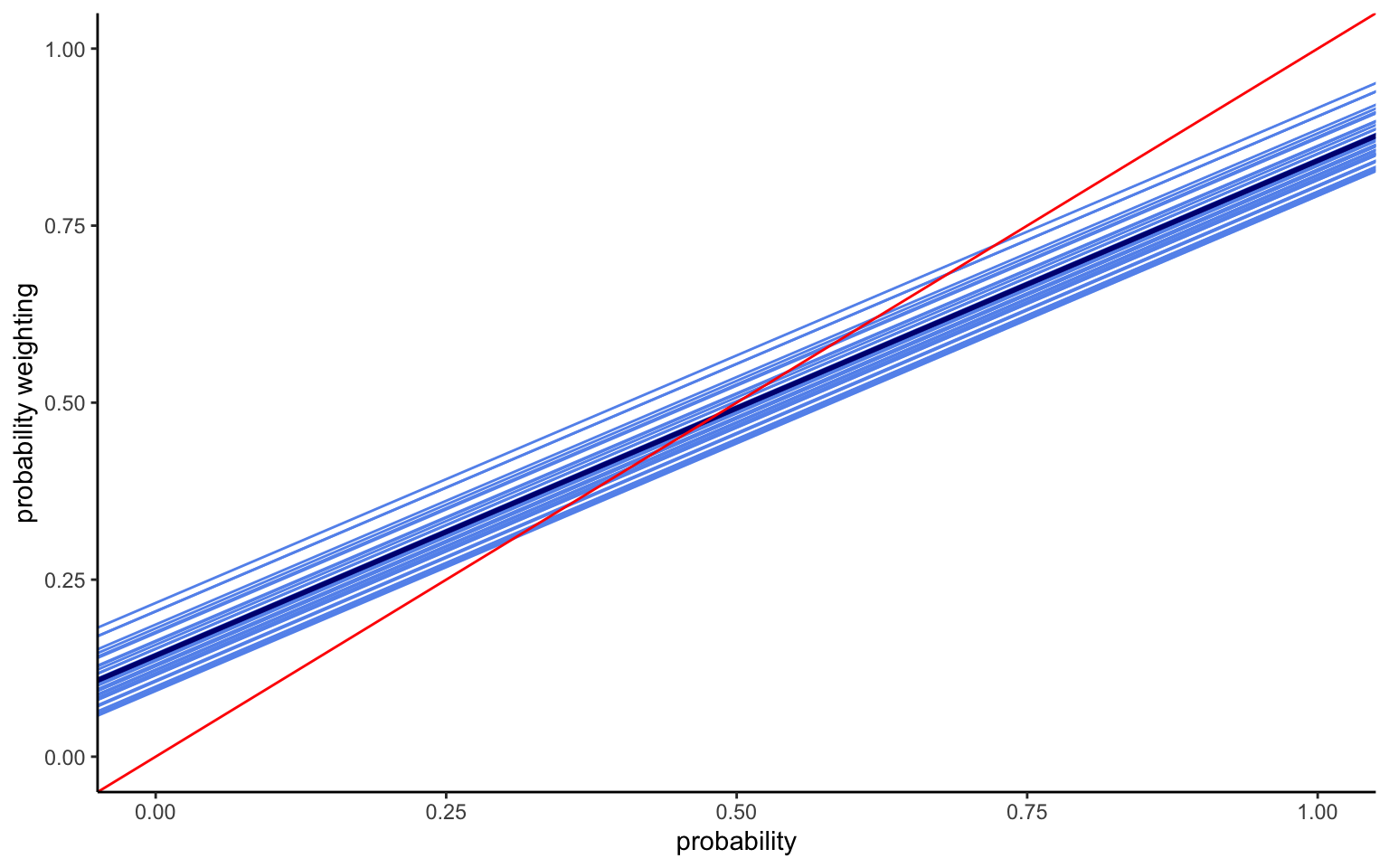
The mean intercept turns out to be the same as before, although this is not necessarily the case, given that the weight for different observations can shift due to the hierarchical structure. The variance is smaller, since we now capture more of the heterogeneity. And indeed, we find significant variation in intercepts between countries, as shown by the value of \(\tau\). The model thus results in a series of parallel lines with different elevations, as shown in Figure 4.1. In terms of interpretation, we thus find very different levels of optimism across the 30 countries.
Once we have allowed for intercepts to differ between countries, however, there is really no reason to force the slope to be the same. We can thus modify the model to allow for a hierarchical slope parameter (sometimes called, random intercepts, random slopes model) in addition to the random intercepts (or hierarchical intercepts—the term “random effects” is best avoided if one wants to publish results in economics, since it triggers memories of panel data models that “one should never use” in economics). Further adding some regularizing hyperpriors to help speeding the estimation along, the Stan code will look as follows:
data{
  int<lower=0> N;
  int<lower=0> Nc;
  vector[N] ce;
  vector[N] p;
  array[N] int ctry;
}
parameters{
  real alpha_hat;
  real beta_hat;
  vector[Nc] alpha;
  vector[Nc] beta;
  real<lower=0> sigma;
  real<lower=0> tau_a;
  real<lower=0> tau_b;
}
model{
// hyperpriors:
alpha_hat ~ std_normal();
beta_hat ~ normal(1,1);
tau_a ~ normal(0,2);
tau_b ~ normal(0,2);

// hierarchical intercepts
  alpha ~ normal(alpha_hat, tau_a);

// hierarchical slopes
  beta ~ normal(beta_hat, tau_b);

// likelihood
for ( i in 1:N )
  ce[i] ~ normal( alpha[ctry[i]] + beta[ctry[i]] * p[i] , sigma  ) ;
}
The code looks much like the one before, with one hierarchical parameter added. However, I now loop through the observations using the for ( i in 1:N ) loop. This avoids issues of dimensionality when multiplying the parameter vector beta (30x1) with the data vector \(p\) (Nx1). We can now estimate the model like before. As a note of caution, this model may run for a little while, depending on the clock speed of your processors. It may thus be desirable to first examine whether we can speed up the model in any way. One possibility may be to parallelize the model to speed it up, but I will not do this here for the sake of clarity of the code. However, a much easier way to speed it up is available by rewriting the loop through the likelihood in vector notation. given the different dimensionality of betaand p, this will require using a “dot-product”, but it is straightforward to implement by replacing the loop with the following line:
ce ~ normal(alpha[ctry] + beta[ctry] .* p, sigma);This simple change to vectorizing the model means that it now runs in about 40% of the time required for the model with the loop.
# creates data to send to Stan
stanD <- list(N = nrow(d30),
              ce = d30$ce_norm,
              p = d30$probability,
              Nc = length(unique(d30$country)),
              ctry = d30$country)

# compile the Stan programme:
sr <- cmdstan_model("stancode/rirs_30countries_vec.stan")

# run the programme:
nm <- sr$sample(
  data = stanD,
  seed = 123,
  chains = 4,
  parallel_chains = 4,
  refresh=200,
  init=0,
  show_messages = TRUE,
  diagnostics = c("divergences", "treedepth", "ebfmi")
)

print(nm, c("alpha_hat","beta_hat","tau_a","tau_b","sigma","alpha","beta"),digits = 3)
nm$save_object(file="stanoutput/rirs_30c.Rds")rirs <- readRDS("stanoutput/rirs_30c.Rds")
print(rirs, c("alpha_hat","beta_hat","tau_a","tau_b","sigma","alpha","beta"),digits = 3) variable mean median sd mad q5 q95 rhat ess_bulk ess_tail
alpha_hat 0.134 0.134 0.015 0.015 0.109 0.159 1.000 6808 2995
beta_hat 0.718 0.718 0.024 0.025 0.678 0.758 1.001 6521 2939
tau_a 0.081 0.080 0.012 0.011 0.064 0.102 1.001 7768 3153
tau_b 0.128 0.127 0.019 0.018 0.102 0.163 1.001 7043 3126
sigma 0.205 0.205 0.001 0.001 0.203 0.206 1.003 5920 2485
alpha[1] 0.076 0.076 0.020 0.021 0.043 0.110 1.000 7736 3209
alpha[2] 0.085 0.085 0.017 0.016 0.057 0.112 1.005 7977 2554
alpha[3] 0.120 0.120 0.018 0.018 0.091 0.148 1.004 7742 2915
alpha[4] 0.187 0.187 0.018 0.018 0.158 0.216 1.001 7542 2900
alpha[5] 0.124 0.124 0.016 0.016 0.097 0.150 1.001 8002 3205
# showing 10 of 65 rows (change via 'max_rows' argument or 'cmdstanr_max_rows' option)p <- as_draws_df(rirs)
zz <- rirs$summary(variables = c("alpha","beta"), "mean" , "sd")
z <- zz %>% separate(variable,c("[","]")) %>%
rename( var = `[`) %>% rename(nid = `]`) %>%
pivot_wider(names_from = var , values_from = c(mean,sd))
ggplot() +
geom_abline(intercept = z$mean_alpha , slope = z$mean_beta, color="cornflowerblue") +
geom_abline(intercept = mean(p$alpha_hat) , slope = mean(p$beta_hat), color="navy" , linewidth=1 ) +
geom_abline(intercept = 0 , slope = 1 , color="red") +
xlim(0,1) + ylim(0,1) + labs(x="probability",y="probability weighting")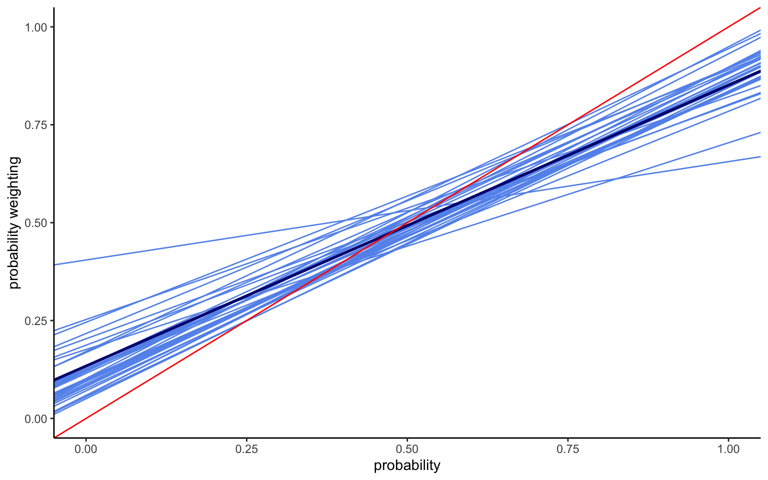
Several things are noteworthy in the results shown in Figure 4.2. We now capture considerable heterogeneity in both the intercept and the slope. The lines thus no longer run parallel to each other. Indeed, providing more flexibility for the slope has increased the variation in intercepts. At the same time, the average intercept has now changed, too, and is somewhat lower than before.
It seems natural to ask whether any difference exists between estimating the global hierarchical model, or estimating the model country by country, or indeed using a fixed effects estimator, which amounts to the same thing (can you see how to implement such a model starting from the code above?). Below, I compare the country-level estimates obtained from the two approaches.
fe <- readRDS("stanoutput/fifs_30c.Rds")
re <- readRDS("stanoutput/rirs_30c.Rds")

p <- as_draws_df(re)

zz <- re$summary(variables = c("alpha","beta"), "mean" , "sd")
zr <- zz %>% separate(variable,c("[","]")) %>%
            rename( var = `[`) %>% rename(nid = `]`) %>%
            pivot_wider(names_from = var , values_from = c(mean,sd))

zz <- fe$summary(variables = c("alpha","beta"), "mean" , "sd")
zf <- zz %>% separate(variable,c("[","]")) %>%
            rename( var = `[`) %>% rename(nid = `]`) %>%
            pivot_wider(names_from = var , values_from = c(mean,sd))

ggplot() +
  geom_point(aes(x=zf$mean_alpha,y=zf$mean_beta,color="Fixed effects estimates"),shape=1,size=3) +
   geom_point(aes(x=zr$mean_alpha,y=zr$mean_beta,color="Bayesian hierarchical estimates"),shape=2,size=3) +
   scale_colour_manual("Legend", values = c("darkgoldenrod","steelblue3","#999999")) +
    geom_vline(xintercept=mean(p$alpha_hat),color="gray",lty="dashed",lwd=1) +
     geom_hline(yintercept=mean(p$beta_hat),color="gray",lty="dashed",lwd=1) +
  labs(x="intercept",y="sensitivity") +
   theme(legend.position = c(0.75, 0.85))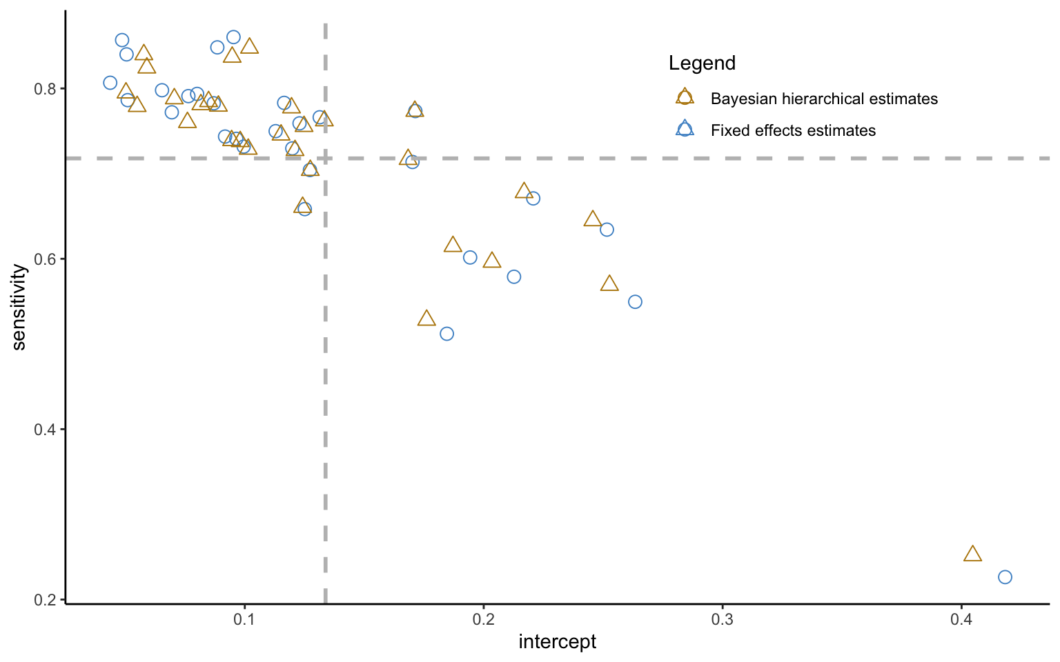
Some striking patterns become apparent in Figure 4.3. For one, the intercept and slope parameters show a strong, negative correlation—a point to which we will return shortly. More interestingly for the question at hand, the estimates from the hierarchical model are not the same as the ones from the fixed effects model. The difference is indeed systematic, with hierarchical estimate being less dispersed about the mean values, indicated by the vertical and horizontal lines. This is shrinkage at work. That is, estimates that fall far from the mean will be shrunk or pooled towards their mean estimate, with the shrinkage increasing in the noisiness of the data. This process follows the exact same equation as the regression to mean observed previously, and once again illustrates the influence of the prior, except that the latter is now endogenously estimated from the aggregate data.
We are now ready to apply the elements seen above to the estimation of nonlinear models. In principle, this application constitutes a straightforward extension of what we have already seen. In practice, however, the estimation of multiple parameters at once—which are often highly constrained to boot—may pose problems for Stan to explore. Luckily, the code can be written using transformed parameters in such a way as to make it much more efficient.
Let us start from a simple EU model, in which only the utility curvature parameter is hierarchical.
data {
 int<lower=1> N;
 int<lower=1> Nid;
 array[N] int id;
 array[N] real ce;
 array[N] real high;
 array[N] real low;
 array[N] real p;
}
parameters {
 vector[Nid] rho;
 real rho_hat;
 real<lower=0> tau;
 real<lower=0> sigma;
}
model {
 vector[N] uh;
 vector[N] ul;
 vector[N] pv;

 rho_hat ~ normal(1,2); // hyperprior for the mean of utility curvature
 tau ~ cauchy(0,5); // hyperprior of variance of rho
 sigma ~ cauchy(0,5); // hyperprior for (aggregate) residual variance

for (n in 1:Nid)
 rho[n] ~ normal(rho_hat , tau); // hierarchical model

for (i in 1:N){
 uh[i] = high[i]^rho[id[i]];
 ul[i] = low[i]^rho[id[i]];
 pv[i] = p[i] * uh[i] + (1-p[i]) * ul[i];
 ce[i] ~ normal( pv[i]^(1/rho[id[i]]) , sigma * high[i] );
 }
}
I use the data from the 2006 Zurich experiment in Bruhin, Fehr-Duda, and Epper (2010) to illustrate the model:
d <- read_csv("data/data_RR_ch06.csv")
dg <- d %>% filter(z1 > 0) %>%
            mutate(high = z1) %>%
            mutate(low = z2) %>%
            mutate(prob = p1) %>%
            group_by(id) %>%
            mutate(id = cur_group_id()) %>%
            ungroup()

pt <- cmdstan_model("stancode/hm_EU.stan")

stanD <- list(N = nrow(dg),
              Nid = max(dg$id),
              id = dg$id,
              high = dg$high,
              low = dg$low,
              p = dg$prob,
              ce = dg$ce)

hm <- pt$sample(
  data = stanD,
  seed = 123,
  chains = 4,
  parallel_chains = 4,
  refresh=200,
  show_messages = FALSE,
  diagnostics = c("divergences", "treedepth", "ebfmi")
)

hm$save_object(file="stanoutput/rr_ch06.Rds")hm <- readRDS("stanoutput/rr_ch06.Rds")
# print aggregate parameters
hm$print(c("rho_hat","tau","sigma"), digits = 3,
"mean", SE = "sd" , "rhat",
~quantile(., probs = c(0.025, 0.975)),max_rows=20) variable mean SE rhat 2.5% 97.5%
rho_hat 1.014 0.039 1.000 0.943 1.094
tau 0.358 0.033 1.022 0.299 0.429
sigma 0.134 0.002 1.004 0.130 0.137# recover individual-level estimates
zz <- hm$summary(variables = c("rho"), "mean" , "sd" )
z <- zz %>% separate(variable,c("[","]")) %>%
rename( var = `[`) %>% rename(id = `]`) %>%
pivot_wider(names_from = var , values_from = c(mean,sd))
# plot distribution
ggplot(z,aes(x=mean_rho)) +
geom_line(stat="density",color="steelblue3",lwd=1) +
geom_vline(xintercept = 1, color="red", lty="dashed") +
xlab("power utility parameter across subjects")
The model above converges readily (it takes about 30 seconds on my laptop). No divergences are produced, and the R-hat statistics look reasonable. It also seems like we are getting a reasonable distribution of parameters, as shown in Figure 4.4. While in practice you will want to look at the standard deviations of the parameters to make sure that they are sufficiently tightly estimated, we will skip this here. Instead, we will consider an alternative way of programming the same model.
The issue is that the model above does not always scale well to multiple parameters. Chances are that even at 2 parameters it will already become problematic. Once you have 3 or more hierarchical parameters, a simple generalization of the model used above will rarely fare well. The model may also behave less well when the parameter to be estimated is highly constrained and many observations fall close to the constraint. The solution in such cases is to reparameterize the model to help Stan explore the posterior distribution. Here, I show how to use a parameter rescaled to follow a standard-normal distribution for the one-parameter model above, before moving on to more complex models.
data {
 int<lower=1> N;
 int<lower=1> Nid;
 array[N] int id;
 array[N] real ce;
 array[N] real high;
 array[N] real low;
 array[N] real p;
}
parameters {
 real rho_hat;
 real<lower=0> tau;
 real<lower=0> sigma;
 array[Nid] real rho_z; //parameter on standard-normal scale
}
transformed parameters{
 vector[Nid] rho;

for (n in 1:Nid){
 rho[n] = rho_hat + tau * rho_z[n]; // mean plus var times rescaled par.
 }
}
model {
 vector[N] uh;
 vector[N] ul;
 vector[N] pv;

 rho_hat ~ normal(1,2);
 tau ~ cauchy(0,5);
 sigma ~ cauchy(0,5);

for (n in 1:Nid)
 rho_z[n] ~ std_normal( ); //prior for rescaled parameters

for (i in 1:N){
 uh[i] = high[i]^rho[id[i]];
 ul[i] = low[i]^rho[id[i]];
 pv[i] = p[i] * uh[i] + (1-p[i]) * ul[i];
 ce[i] ~ normal( pv[i]^(1/rho[id[i]]) , sigma * high[i] );
 }
}
You can see the re-parameterized model above. The data block has remained unchanged. The parameter block now contains a new variable rho_z instead of rho, which rho instead being declared in the transformed parameters block. Notice also that I now specify rho_z as an array instead of a vector. This is not hugely important here, but will make the code more efficient down the road. A second—and indeed crucial—point is that, other than rho above, rho_z is now rescaled: relative to the parameter rho, it is demeaned and multiplied by the standard deviation of the parameter, which ensures that it will follow a standard-normal distribution (which is indeed used as a prior in the model block). Given this new writing of the model, the aggregate parameters are now specified in the transformed parameters block. While this way of writing the model may seem backwards at first, it can yield substantial improvements in estimation speed, and for more complex models, may well make the difference between a model that converges and one that does not.
d <- read_csv("data/data_RR_ch06.csv")

dg <- d %>% filter(z1 > 0) %>%
            mutate(high = z1) %>%
            mutate(low = z2) %>%
            mutate(prob = p1) %>%
            group_by(id) %>%
            mutate(id = cur_group_id()) %>%
            ungroup()

pt <- cmdstan_model("stancode/hm_EU_resc.stan")

stanD <- list(N = nrow(dg),
              Nid = max(dg$id),
              id = dg$id,
              high = dg$high,
              low = dg$low,
              p = dg$prob,
              ce = dg$ce)

hm <- pt$sample(
  data = stanD,
  seed = 123,
  chains = 4,
  parallel_chains = 4,
  refresh=500,
  show_messages = FALSE,
  diagnostics = c("divergences", "treedepth", "ebfmi")
)

hm$save_object(file="stanoutput/rr_ch06_resc.Rds")hm <- readRDS("stanoutput/rr_ch06.Rds")
# print aggregate parameters
hm$print(c("rho_hat","tau","sigma"), digits = 3,
"mean", SE = "sd" , "rhat",
~quantile(., probs = c(0.025, 0.975)),max_rows=20) variable mean SE rhat 2.5% 97.5%
rho_hat 1.014 0.039 1.000 0.943 1.094
tau 0.358 0.033 1.022 0.299 0.429
sigma 0.134 0.002 1.004 0.130 0.137# recover individual-level estimates
zz <- hm$summary(variables = c("rho"), "mean" , "sd" )
z <- zz %>% separate(variable,c("[","]")) %>%
rename( var = `[`) %>% rename(id = `]`) %>%
pivot_wider(names_from = var , values_from = c(mean,sd))
# plot distribution
ggplot(z,aes(x=mean_rho)) +
geom_line(stat="density",color="steelblue3",lwd=1) +
geom_vline(xintercept = 1, color="red", lty="dashed") +
xlab("power utility parameter across subjects")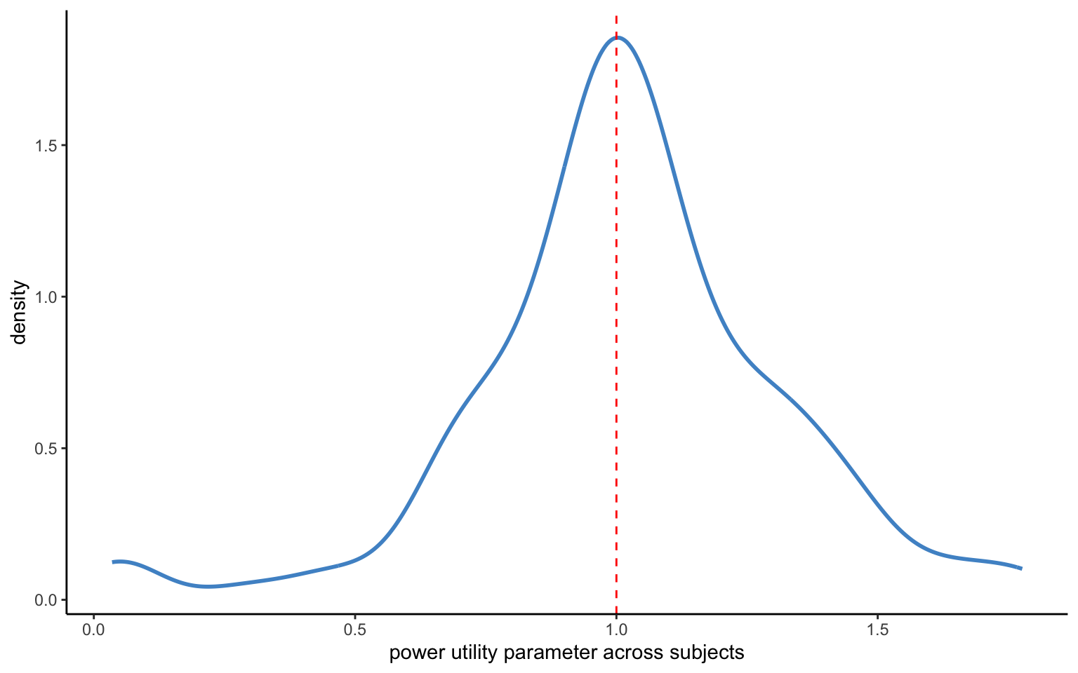
Let us go ahead and estimate the model now. Again, there are no divergences, and the R-hats on the aggregate level parameters look good. The distribution of the individual-level means looks much like before. The model now converges in some 20 seconds on my laptop, instead of the 34 seconds of the previous model. While this improvement may not look like much, it amounts to close to a 40% speed gain. Once we are dealing with models that take hours or days to converge, that can make a real difference. The distribution of individual-level parameters in Figure 4.5 looks almost exactly the same as before.
With the decentralized model above in hand, it is now straightforward to build a model with multiple hierarchical parameters. Let us again use the same data, and let us build a PT model, restricted to gains only for simplicity (adding additional parameters for losses is straightforward). First, we will want to change the model to include a probability weighting function. Making the error term hierarchical, too, yields 4 hierarchical parameters.
Next, we get to work on the transformed parameters block. Instead of using an array rho, I introduce an element pars made up of an array of vectors. This will allow us to loop through vectors of the 4 parameters in the subsequent code. Do not forget to actually create the vectors of parameters. In place of rho_hat, we now use a 4-dimensional vector called means, since the dimensionality of the different elements in the loop needs to line up for the code to work. I now furthermore restrict all parameters to be positive (although for rho this is ot strictly necessary) by defining them as the exponential of the corresponding element in pars. Finally, don’t forget to give hyperpriors to the aggregate means, keeping in mind that they are expressed on a transformed scale.
Since we have 4 parameters, tau now becomes a vector of parameter variances. The diag_matrix function maps this vector into a matrix, i.e. it creates a matrix \(\tau \times \text{I}\), where \(\text{I}\) is an indentity matrix with the same number of rows and columns as hierarchical parameters in the model. What used to be rho_z becomes an array of vectors, which we simply call Z. Note that it needs to be indexed by the subject identifier n in the loop, which extracts one vector at the time, thus ensuring again that all expressions have the same dimension. We then obtain the original parameters of interest as usual, by defining them based on the transformed parameter line, and applying the appropriate constraints. Note that we could of course also define every parameter using a separate line, following the code used for utility curvature above. Using matrix notation like done here, however, makes the code more compact and prepares the ground for the estimation of covariance matrices of the parameters, which we will develop shortly.
data {
 int<lower=1> N;
 int<lower=1> Nid;
 array[N] int id;
 array[N] real ce;
 array[N] real high;
 array[N] real low;
 array[N] real p;
}
parameters {
 vector[4] means;
 vector<lower=0>[4] tau;
 array[Nid] vector[4] Z;
}
transformed parameters{
 array[Nid] vector[4] pars;
 vector<lower=0>[Nid] rho;
 vector<lower=0>[Nid] gamma;
 vector<lower=0>[Nid] delta;
 vector<lower=0>[Nid] sigma;
for (n in 1:Nid){
 pars[n] = means + diag_matrix(tau) * Z[n];
 rho[n] = exp( pars[n,1] );
 gamma[n] = exp( pars[n,2] );
 delta[n] = exp( pars[n,3] );
 sigma[n] = exp( pars[n,4] );
 }
}
model {
 vector[N] uh;
 vector[N] ul;
 vector[N] pw;
 vector[N] pv;

 means[1] ~ normal(0,1);
 means[2] ~ normal(0,1);
 means[3] ~ normal(0,1);
 means[4] ~ normal(0,1);
 tau ~ exponential(5);

for (n in 1:Nid)
 Z[n] ~ std_normal( );

for (i in 1:N){
 uh[i] = high[i]^rho[id[i]];
 ul[i] = low[i]^rho[id[i]];
 pw[i] = (delta[id[i]] * p[i]^gamma[id[i]])/
         (delta[id[i]] * p[i]^gamma[id[i]] + (1 - p[i])^gamma[id[i]]);
 pv[i] = pw[i] * uh[i] + (1-pw[i]) * ul[i];
 ce[i] ~ normal( pv[i]^(1/rho[id[i]]) , sigma[id[i]] * (high[i] - low[i]) );
 }
}d <- read_csv("data/data_RR_ch06.csv")
dg <- d %>% filter(z1 > 0) %>%
mutate(high = z1) %>%
mutate(low = z2) %>%
mutate(prob = p1) %>%
group_by(id) %>%
mutate(id = cur_group_id()) %>%
ungroup()
pt <- cmdstan_model("stancode/hm_RDU_var.stan")
stanD <- list(N = nrow(dg),
Nid = max(dg$id),
id = dg$id,
high = dg$high,
low = dg$low,
p = dg$prob,
ce = dg$ce)
hm <- pt$sample(
data = stanD,
seed = 123,
chains = 4,
parallel_chains = 4,
refresh=200,
adapt_delta = 0.99,
max_treedepth = 15,
show_messages = FALSE,
diagnostics = c("divergences", "treedepth", "ebfmi")
)
#257.0 seconds
hm$save_object(file="stanoutput/RR_ch6_RDU_var.Rds")We are now ready to estimate the model. To do this, it will be wise to lower the stepsize to small values using the adapt_delta option—a value of 0.99 is typically recommended. At the same time, let us allow for a larger value of max_treedepth (the default is 10), which means that the algorithm may explore for longer. Both these tunings are made necessary by the highly nonlinear nature of the model, which creates parameter regions that are tricky to explore. Even so, such models may on occasion produce a small number of divergences. This is not unusual in highly nonlinear models such as this one. You would nevertheless be well advised to check the convergence statistics in depth, especially for new models that you have never used before.
hm <- readRDS("stanoutput/RR_ch6_RDU_var.Rds")

# print aggregate parameters
hm$print(c("means","tau"), digits = 3,
          "mean", SE = "sd" , "rhat",
         ~quantile(., probs = c(0.025, 0.975)),max_rows=20)
variable mean SE rhat 2.5% 97.5%
means[1] -0.068 0.020 1.002 -0.109 -0.031
means[2] -0.773 0.041 1.002 -0.852 -0.694
means[3] -0.171 0.032 1.001 -0.235 -0.108
means[4] -2.364 0.050 1.003 -2.462 -2.264
tau[1] 0.083 0.035 1.012 0.011 0.149
tau[2] 0.418 0.034 1.001 0.358 0.489
tau[3] 0.290 0.025 1.001 0.243 0.341
tau[4] 0.523 0.040 1.002 0.451 0.608# recover individual-level estimates
zz <- hm$summary(variables = c("rho","gamma","delta","sigma"), "mean" , "sd" )
z <- zz %>% separate(variable,c("[","]")) %>%
rename( var = `[`) %>% rename(id = `]`) %>%
pivot_wider(names_from = var , values_from = c(mean,sd))
# plot distribution
ggplot(z,aes(x=mean_gamma)) +
geom_line(stat="density",color="steelblue3",lwd=1) +
geom_vline(xintercept = 1, color="red", lty="dashed") +
xlab("likelihood-insensitivity across subjects")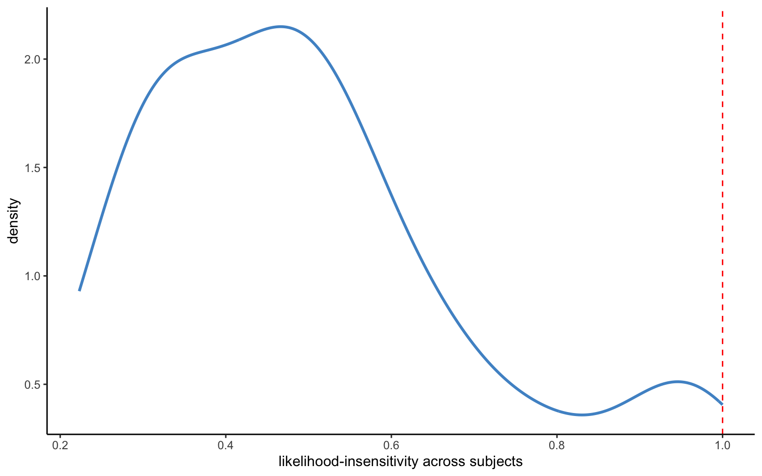
Figure 4.6 shows the distribution of the means of individual-level likelihood-sensitivity parameters. The means are somewhat difficult to interpret, since they are on a transformed scale (and in any case, we may want to examine the means or medians of the individual-level parameters instead). The standard deviations of the individual-level estimates seem to be suitably small, indicating a fairly good identification of the parameters, although there is also quite some heterogeneity between subjects.
The model above works perfectly fine in estimating the desired PT parameters. It does, however, treat the various model parameters as independent from each other. From a Bayesian point of view—if there is some correlation between the parameters—then we should be able to improve our estimations by explicitly modelling the co-variation structure between the parameters. This is due as usual to the posterior uncertainty about the true parameters. To illustrate, we can use the fixed-effects (individual-level) estimates on the data of Bruhin et al. discussed in chapter 2. I display them again here below for easy access. A remarkable feature of the data is that likelihood-sensitivity and the residual error are strongly negatively correlated (with subject nr. 9 constituting a noteworthy outlier). Such correlations indeed also occur between other model parameters—Vieider (2024) provides a theoretical account showing what may be behind this.
knitr::include_graphics('figures/scatter_RR.png')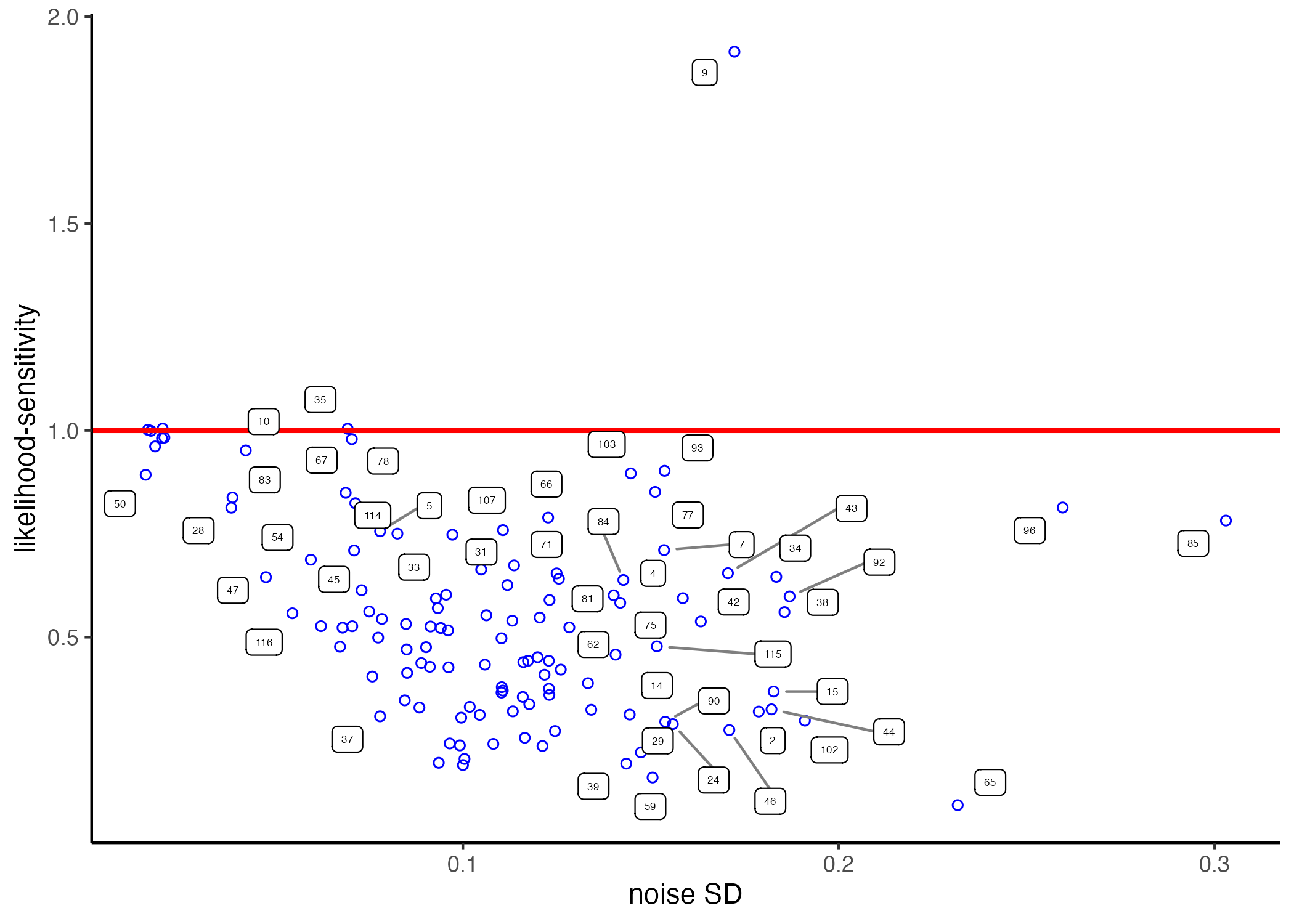
We will now try to leverage this additional information by estimating a model including a covariance matrix between all the different model parameters. The change to the model needed to achieve this—displayed below—is fairly trivial. We simply replace the diag_matrix containing the parameter variance vector, with the diag_pre_multiply matrix. The latter contains the parameter variance vector, and a Cholesky-decomposed covariance matrix. Of course, we give that matrix an appropriate prior, following best practices as recommended by the Stan community. For good measure we also define a transformed parameter Rho, which recovers the correlation parameters on the original scale (this could of course also be done post-estimation in R, or we could specify the same line of code in the generated quantities block, since it is not used in the estimations).
data {
 int<lower=1> N;
 int<lower=1> Nid;
 array[N] int id;
 array[N] real ce;
 array[N] real high;
 array[N] real low;
 array[N] real p;
}
parameters {
 vector[4] means;
 vector<lower=0>[4] tau;
 array[Nid] vector[4] Z;
 cholesky_factor_corr[4] L_omega;
}
transformed parameters{
 matrix[4,4] Rho = L_omega*transpose(L_omega);
 array[Nid] vector[4] pars;
 vector<lower=0>[Nid] rho;
 vector<lower=0>[Nid] gamma;
 vector<lower=0>[Nid] delta;
 vector<lower=0>[Nid] sigma;
for (n in 1:Nid){
 pars[n] = means + diag_pre_multiply(tau, L_omega) * Z[n];
 rho[n] = exp( pars[n,1] );
 gamma[n] = exp( pars[n,2] );
 delta[n] = exp( pars[n,3] );
 sigma[n] = exp( pars[n,4] );
 }
}
model {
 vector[N] uh;
 vector[N] ul;
 vector[N] pw;
 vector[N] pv;

 means[1] ~ normal(0,1);
 means[2] ~ normal(0,1);
 means[3] ~ normal(0,1);
 means[4] ~ normal(0,1);
 tau ~ exponential(5);
 L_omega ~ lkj_corr_cholesky(4);

for (n in 1:Nid)
 Z[n] ~ std_normal( );

for (i in 1:N){
 uh[i] = high[i]^rho[id[i]];
 ul[i] = low[i]^rho[id[i]];
 pw[i] = (delta[id[i]] * p[i]^gamma[id[i]])/
         (delta[id[i]] * p[i]^gamma[id[i]] + (1 - p[i])^gamma[id[i]]);
 pv[i] = pw[i] * uh[i] + (1-pw[i]) * ul[i];
 ce[i] ~ normal( pv[i]^(1/rho[id[i]]) , sigma[id[i]] * (high[i] - low[i]) );
 }
}d <- read_csv("data/data_RR_ch06.csv")
dg <- d %>% filter(z1 > 0) %>%
mutate(high = z1) %>%
mutate(low = z2) %>%
mutate(prob = p1) %>%
group_by(id) %>%
mutate(id = cur_group_id()) %>%
ungroup()
pt <- cmdstan_model("stancode/hm_RDU.stan")
stanD <- list(N = nrow(dg),
Nid = max(dg$id),
id = dg$id,
high = dg$high,
low = dg$low,
p = dg$prob,
ce = dg$ce)
hm <- pt$sample(
data = stanD,
seed = 123,
chains = 4,
parallel_chains = 4,
refresh=200,
adapt_delta = 0.99,
max_treedepth = 15,
show_messages = FALSE,
diagnostics = c("divergences", "treedepth", "ebfmi")
)
#841.9 seconds
hm$save_object(file="stanoutput/RR_ch6_RDU.Rds")Figure 4.7 plots the likelihood-sensitivity parameter from the model with variances only against the one including the covariance matrix. Most of the parameters are virtually the same. This is reassuring, inasmuch as we would not expect the covariance matrix to fundamentally affected our inferences. However, especially the estimates falling into the fourth quartile of the residual variance—i.e. the observations with the largest noise—can be seen to be adjusted downwards. This happens because large error variance is associated with low likelihood-sensitivity, which is exactly the effect that most strongly emerges from the correlation matrix. Using this information, the model thus corrects observations indicating strong likelihood-sensitivity with little confidence downwards, to maximize predictive performance.
hc <- readRDS(file="stanoutput/RR_ch6_RDU.Rds")
hv <- readRDS(file="stanoutput/RR_ch6_RDU_var.Rds")

zz <- hc$summary(variables = c("rho","gamma","delta","sigma"), "mean" , "sd" )
zc <- zz %>% separate(variable,c("[","]")) %>%
            rename( var = `[`) %>% rename(id = `]`) %>%
            pivot_wider(names_from = var , values_from = c(mean,sd)) %>%
            rename(gamma_c = mean_gamma,rho_c = mean_rho,delta_c = mean_delta,sigma_c = mean_sigma)

zz <- hv$summary(variables = c("rho","gamma","delta","sigma"), "mean" , "sd" )
zv <- zz %>% separate(variable,c("[","]")) %>%
            rename( var = `[`) %>% rename(id = `]`) %>%
            pivot_wider(names_from = var , values_from = c(mean,sd)) %>%
            rename(gamma_v = mean_gamma,rho_v = mean_rho,delta_v = mean_delta,sigma_v = mean_sigma)

z <- left_join(zc,zv,by="id")
z <- z %>% mutate(qs = ntile(sigma_v,4))

ggplot(z,aes(x=gamma_v,y=gamma_c,color=as.factor(qs))) +
  geom_point() +
  geom_abline(intercept=0,slope=1,color="red") +
  #geom_vline(xintercept=mean(z$gamma_v)) +
  geom_label_repel(aes(label = id),
                  box.padding   = 0.35,
                  point.padding = 0.5,
                  size          = 1.5,
                  segment.color = 'grey50') +
  scale_colour_manual("Error quartile", values = c("black","darkgoldenrod","#999999","steelblue3")) +
  theme(legend.position = c(0.25, 0.8))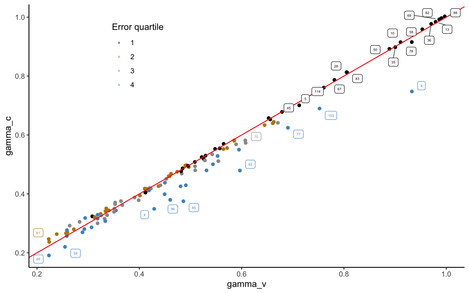
A particularly strong adjustment can be seen for subject 9. Figure 4.8 shows three probability weighting functions fit to the datapoints for subject 9 in the Zurich 2006 data of Bruhin et al.—a function based on individual-level estimation (fixed effects); a function based on the hierarchical model with variance only; and a function based on the hierarchical model including the covariance matrix. The fixed effect model seems to provide the best fit to the nonparametric data. However, this fit seems only slightly better than the one of the hierarchical estimate with variance only, which changes our inference from the subject being oversensitive to probabilities to being slightly insensitive. Indeed, a closer look reveals that the hierarchical estimate—even though it is (slightly) inverse S-shaped instead of S-shaped—may not be statistically different from the fixed effect estimate, which carries very low confidence, as shown by the wide variation in the posterior draws, indicated by the light grey lines (made up of 200 randomly drawn rowns of the posterior).
# load fixed effects estimate
hf <- readRDS(file="stanoutput/ind_ZCH06_fixed.RDS")

zz <- hf$summary(variables = c("rho","gamma","delta","sigma"), "mean" , "sd")
zf <- zz %>% separate(variable,c("[","]")) %>%
            rename( var = `[`) %>% rename(id = `]`) %>%
            pivot_wider(names_from = var , values_from = c(mean,sd)) %>%
            rename(rho = mean_rho , gamma = mean_gamma , delta = mean_delta , sigma = mean_sigma)

# load hierarchical estimate with covar
hc <- readRDS(file="stanoutput/RR_CH6_RDU.Rds")

zz <- hc$summary(variables = c("rho","gamma","delta","sigma"), "mean" , "sd")
zc <- zz %>% separate(variable,c("[","]")) %>%
            rename( var = `[`) %>% rename(id = `]`) %>%
            pivot_wider(names_from = var , values_from = c(mean,sd)) %>%
            rename(rho = mean_rho , gamma = mean_gamma , delta = mean_delta , sigma = mean_sigma)


# load hierarchical estimate with var only
hv <- readRDS(file="stanoutput/RR_CH6_RDU_var.Rds")
zzv <- hv$summary(variables = c("rho","gamma","delta","sigma"), "mean" , "sd")
zv <- zzv %>% separate(variable,c("[","]")) %>%
            rename( var = `[`) %>% rename(id = `]`) %>%
            pivot_wider(names_from = var , values_from = c(mean,sd)) %>%
            rename(rho = mean_rho , gamma = mean_gamma , delta = mean_delta , sigma = mean_sigma)


d <- read_csv("data/data_rr_ch06.csv")
dg9 <- d %>% filter(z1 > 0) %>%
            mutate(high = z1) %>%
            mutate(low = z2) %>%
            mutate(prob = p1) %>%
            group_by(id) %>%
            mutate(id = cur_group_id()) %>%
            ungroup() %>%
            filter(id==9) %>%
            mutate( dw = (ce - low)/(high - low) ) %>%
            group_by(prob,high,low) %>%
            mutate(mean_dw = mean(dw)) %>%
            mutate(median_dw = median(dw)) %>%
            ungroup()

###
d9 <- as_draws_df(hf)
g9 <- d9$`gamma[9]`
de9 <- d9$`delta[9]`
r9 <- as.data.frame(cbind(g9,de9))

r9 <- r9 %>% sample_n(size=200) %>%
               mutate(row = row_number())

fe9 <- function(x) (zf$delta[id=9] * x^zf$gamma[id=9] / (zf$delta[id=9] * x^zf$gamma[id=9] + (1-x)^zf$gamma[id=9]))
hm9 <- function(x) (zc$delta[id=9] * x^zc$gamma[id=9] / (zc$delta[id=9] * x^zc$gamma[id=9] + (1-x)^zc$gamma[id=9]))
hm9v <- function(x) (zv$delta[id=9] * x^zv$gamma[id=9] / (zv$delta[id=9] * x^zv$gamma[id=9] + (1-x)^zv$gamma[id=9]))
ggplot() +
   purrr::pmap(r9, function(de9,g9, row) {
    stat_function( fun = function(x) ( de9*x^g9 )/( de9*x^g9 + (1-x)^g9) ,
                   color="grey" , linewidth = 0.25)
    }) +
  stat_function(fun = fe9,aes(color="fixed effect"),linewidth=1) + xlim(0,1) +
  stat_function(fun = hm9,aes(color="hierarchical covar."),linewidth=1) +
  stat_function(fun = hm9v,aes(color="hierarchical"),linewidth=1) +
  geom_point(aes(x=dg9$prob,y=dg9$mean_dw),size=3, color="chartreuse4",shape=10) +
  geom_abline(intercept=0, slope=1,linetype="dashed",color="gray") +
  scale_colour_manual("Legend", values = c("steelblue3","darkgoldenrod", "chocolate4")) +
    xlab("probability") + ylab("decision weights") + theme(legend.position = c(0.8, 0.2))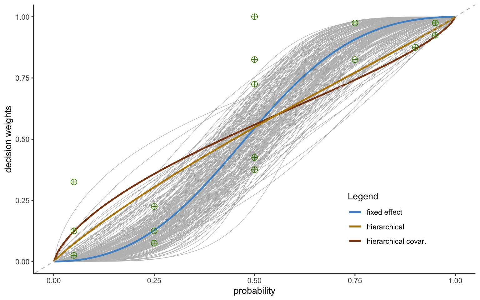
Most importantly, however, the hierarchical function reflects the fact that this particular observation seems unlikely, given the distribution of parameters in the population. Since the estimate is furthermore very noisy, it is shrunk towards the population mean. This follows standard Bayesian procedures, whereby noisy outliers are discounted and drawn towards the prior, which in this case is endogenously estimated from the aggregate data (see BOX for a short discussion). Such shrinkage serves to optimize predictive performance, and is based on the probability distributions gathered from the environment.
Take a parameter \(\gamma\) that is distributed \(\gamma_i \sim \mathcal{N}(\widehat{\gamma}_i,\sigma_i^2)\), where \(\widehat{\gamma}_i\) indicates the true parameter mean to be estimated for subject \(i\), whereas \(\gamma_i\) is the maximum likelihood estimator (individual fixed effect). The two may not coincide, for instance because of large sampling variation in small samples. Assume further that the prior distribution of this estimator in the population is also normal, so that \(\widehat{\gamma} \sim \mathcal{N}(\mu,\tau^2)\). The Bayesian posterior will then itself follow a normal distribution, with mean \(\widehat{\gamma}_i = \frac{\sigma^2}{\sigma^2 + \tau^2}\gamma_i + \frac{\tau^2}{\sigma^2 + \tau^2}\mu\) and variance \(\frac{\sigma_i^2\tau^2}{\sigma_i^2 + \tau^2} = \frac{1}{\sigma_i^2} + \frac{1}{\tau^2}\). That is, the posterior mean will be a convex combination of the fixed effect estimator and the prior mean. The “shrinkage weight” \(\frac{\sigma^2}{\sigma^2 + \tau^2} = 1 - \frac{\tau^2}{\sigma^2 + \tau^2}\) will be a function of the variance of the parameter itself, and of the prior variance. The larger the variance of the individual parameter, the lower the weight attributed to it, and the larger the weight attributed to the prior mean. The greater the population variance \(\sigma^2\), the less weight is attributed to the prior mean, capturing the intuition that outliers from more homogeneous populations are discounted more. Notice that these equations are directly applicable to our calculations for subject 9. We have \(\gamma_9 = 2.08\), \(\sigma_9^2 = 0.36\), \(\mu = 0.45\), and \(\tau^2 = 0.16\). We thus obtain \(\widehat{\gamma}_9 =\) 0.9515385. The value estimated from the hierarchical model is very similar at 0.934. Note, however, that including a covariance matrix further lowers this value to 0.73. This is due to the more complex structure implemented in the estimated model, which takes into account the strongly negative correlation between likelihood-sensitivity and noise.
This is particularly apparent from the function estimated from the hierarchical model including a covariance matrix. The latter indeed seems to fall even farther from the fixed effects estimator, and is now arguably statistically distinct from it at conventional levels taken to indicate significance. Nevertheless, it appears the most likely function in the context of the entirety of the data, incorporating not only the likelihood of any given parameter value based on the parameter distribution in the population, but also the correlation structure between the different parameters in the model. Note that these large differences emerge because the outlier is noisy—perfectly identified outliers will not be shrunk.
Covariance matrices can thus be a great way of improving the information content in hierarchical models. Nevertheless, some caution is called for. In particular, there can be circumstances where a covariance matrix does more harm than good. This will for instance occur in data with large, low-noise outliers. Such outliers may then distort the parametric correlations in the matrix, in extreme cases even in the opposite direction of the nonparametric correlations observed between estimated parameters. It is thus always a good idea to check the correlations in both ways (i.e., to compare the parametric estimation in the matrix to rank-correlations of the posterior means of the individual-level parameters). While some quantitative differences are expected, wildly differing correlation coefficients that may even go in opposite directions are a sign of trouble afoot.
Often we will want to conduct regression analysis using the parameters of the decision model as dependent variables (or indeed as independent variables). It may be tempting to simply estimate the model, obtain the posterior means of the individual-level parameters, and then to conduct the regression analysis using these parameter means using standard regression tools. Such a procedure, however, has the distinct drawback of throwing away the information on the confidence we have in the different estimates. Given large variation in the reliability of estimates, that may severely bias our ultimate inferences. Here, I discuss how to conduct regression analysis in such a way as to consider the full posterior uncertainty about the parameter estimates. (In some cases, this method may not be applicable, e.g. because the original data are not available. In this case, one could approximate this procedure using a measurement error model—see the end of the following section for details).
Let us look at this based on the PT model with covariance matrix from above. Assume you want to regress the likelihood-sensitivity parameter, \(\gamma\), on some demographics, say sex and age. Just like in linear regression models discussed in chapter 2, it will be convinient to add these demographics to a design matrix, x, together with a column of 1s to model the intercept. All that is then required is to add the following line below the loop estimating the model parameters (of course, you will also need to import the design matrix x in the data block and declare its dimensions; and to declare the vector of regression coefficients beta and the scale parameter of the regression tau in the parameters block): gamma ~ normal( x * beta , tau);.
We are now conducting a regression of the parameter, which is automatically treated as an uncertain quantity. That is, writing the regression equation like this will take the full posterior uncertainty about gamma into account. The code here below executes a regression of likelihood-sensitivity on sex (specifically, a female dummy) and on the semester of study (for no other reason than that there are not many other variables available in the data set).
d <- read_csv("data/data_RR_ch06.csv")

dg <- d %>% filter(z1 > 0) %>%
            mutate(high = z1) %>%
            mutate(low = z2) %>%
            mutate(prob = p1) %>%
            group_by(id) %>%
            mutate(id = cur_group_id()) %>%
            ungroup()

pt <- cmdstan_model("stancode/hm_RDU_reg.stan")

di <- dg %>% group_by(id) %>%
             filter(row_number()==1) %>%
             ungroup()

x <- model.matrix( ~ female + semester, di)

stanD <- list(N = nrow(dg),
              Nid = max(dg$id),
              id = dg$id,
              high = dg$high,
              low = dg$low,
              p = dg$prob,
              ce = dg$ce,
              K = ncol(x),
              x = x)

hm <- pt$sample(
  data = stanD,
  seed = 123,
  chains = 4,
  parallel_chains = 4,
  refresh=200,
  adapt_delta = 0.99,
  max_treedepth = 15,
  show_messages = TRUE,
  init = 0,
  diagnostics = c("divergences", "treedepth", "ebfmi")
)


hm$save_object(file="stanoutput/RR_ch6_RDU_reg.Rds")hm <- readRDS("stanoutput/RR_ch6_RDU_reg.Rds")
hm$print(c("beta"), digits = 3,
"mean", SE = "sd" , "rhat",
~quantile(., probs = c(0.025, 0.975)),max_rows=30) variable mean SE rhat 2.5% 97.5%
beta[1] 0.529 0.033 1.000 0.464 0.595
beta[2] -0.106 0.034 1.000 -0.170 -0.039
beta[3] 0.003 0.007 1.000 -0.010 0.016The results indicate that females display less likelihood-sensitivity—a common finding in the literature, see e.g. L’Haridon and Vieider (2019). In most practical applications, however, you will want to regress all the parameters at once on the independent variables of interest. A very simple way of coding this would be to add a line of code for each separate parameter into the model (and of course to declare as many scale parameters and regression coefficient vectors). Alternatively, one could collect all the parameters into a matrix and run all the regressions at once. The principle is however the same as above, so that generalizing this model is left as an exercise. Of course, this is not the only way of incorporating regressions into the model. It is, however, particularly flexible, allowing for recombinations of (full posteriors of) parameters, and to include parameter e.g. as right-hand side controls, instead of as dependent variables as shown above.
Meta-analysis is nothing but a hierarchical analysis where the lowest level is encoded from existing studies, i.e. we directly obtain the mean and standard deviation (standard error in frequentist terms) of the variable of interest. Beyond standard meta-analytic applications, the model is thus suitable in any situation in which one may wish to obtain aggregate estimates across several instances in which an effect is measured with error. This may for instance apply to the case where (almost) identical experiments are executed in a number of different locations. In such cases, the method will deliver several desirable outcomes at once—obtaining an aggregate estimate; correcting individual estimates for measurement error; disciplining multiple tests by explicitly modelling their inter-dependence; and correcting local inferences from the single experiments by making use of the global information provided by all the data. The usual caveat applies—this is not a textbook in meta-analysis, and such a textbook should be consulted for many important details. Here, I will rather focus on the technical details required to implement meta-analysis in Stan.
Let us start from an example based on the clinical trial data from table 5.4 in BDA3 to illustrate the approach. Technically, the data summarize the effect of beta-blockers on reducing mortality after myocardial infarction. The data have been collected in 22 hospitals, and we have data on the log-odds and the associated standard errors, which can be assumed to be approximately normally distributed. Beyond these details, however, the data could be anything, and you might think of them as risk taking tendencies in 22 experiments, or indeed as the effect of a nudging intervention on some sort of behaviour.
bb <- data.frame(log_odds  = c("0.028","-0.741","-0.541","-0.246","0.069","-0.584",
                               "-0.512","-0.079","-0.424","0.335","-0.213","-0.039",
                               "-0.593","0.282","-0.321","-0.135","0.141","0.322","0.444",
                               "-0.218","-0.591","-0.608"),
                         sd = c("0.850","0.483","0.565","0.138","0.281","0.676","0.139","0.204",
                                "0.274","0.117","0.195","0.229","0.425","0.205","0.298",
                                "0.261","0.364","0.553","0.717","0.260","0.257","0.272"))
bb <- as.data.frame(apply(bb, 2, as.numeric))
bb <- bb %>% mutate( lower = log_odds - 1.96*sd ) %>%
             mutate( upper = log_odds + 1.96*sd ) %>%
             mutate(study = row_number())
We can display these data in a graph as follows:
ggplot(data=bb, aes(y=study, x=log_odds, xmin=lower, xmax=upper)) +
  geom_point(size=2,color="cornflowerblue") +
  geom_errorbarh(height=.1,color="cornflowerblue") +
  geom_vline(xintercept=0,color="red",linetype="dashed") +
  scale_y_continuous(name = "", breaks=1:nrow(bb), labels=bb$study)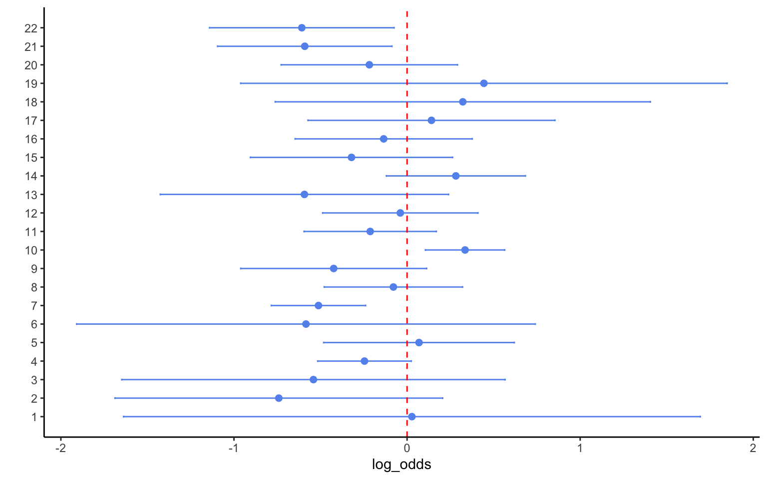
The graph shows that most of the effects were not significant, i.e. Beta blockers do not seem to reduce the likelihood of myocardial infarction based on most of these studies. Three studies had a significantly negative effect, suggesting that the intervention worked. However, one study recorded a significantly positive effect, suggesting that the intervention made the disease worse. Given evidence like this, most traditional literature reviews would conclude that there is no effect. Even tallying up significant effects, as some scholars have done, would not yield any clear insights here. At the very least, a systematic Bayesian analysis should allow us to describe the evidence somewhat better.
First, however, we need to check whether the conditions are fulfilled under which we can apply Bayesian hierarchical analysis to the problem. Given that we know nothing about the 22 hospitals, we should consider them as exchangeable—an important condition for a hierarchical model (Note: if we were aware of some characteristics that might matter, say the size of the hospital or the prevalence of the disease in the city where the hospital is located, we could control for this in a regression, so that the observations would again become exchangeable conditional on size and disease prevalence). We should also make sure that the experiments were comparable, though in the absence of evidence to the contrary we may well choose to assume so. We are thus good to go.
The basic assumption underlying a meta-analysis (or for that matter, any measurement error model) is that we might not be observing the true effect size in single experiments. The reasons for that can vary. Perhaps the most standard reason is that, according to sampling theory, we would approximate the true effect size only as the sample size tends to infinity. Any small subsample may thus be affected by sampling error. Sampling error can be increased by all sorts of other errors, including (unobserved) randomization failures, measurement or recording errors, unobserved differences between locations and implementation protocols and the like. We will thus model the observed log-odds, \(x\), as being distributed normally, with as their mean the true (but unobserved) log odds, \(\widehat{x}\), and with the standard deviation given by the observed standard error: \[ x_i \sim \mathcal{N}(\widehat{x}_i \, , \, se_i), \] where I have subscriped the quantities by \(i\) to emphasize that they belong to the ith experiment. We will further model the true effect sizes as being drawn from a common mean \(\mu\), and following some distribution around that mean that captures the “true variation” in effect sizes that is not due to error. This is indeed the very reason to model the effect hierarchically—after all, if we were sure that all experiments were truly identical, we could simply pool the data. Each study will enter this equation with a weight that is proportional to the inverse of its variance (i.e. it will receive a weight \(\frac{\sigma^2}{\sigma^2 + se_i^2}\) in a normal-normal model as above). The Stan code below implements such a model using vector notation.
data{
    int<lower=1> N;
    vector[N] lo;
    vector[N] se;
}
parameters{
    vector<lower=0>[N] lo_hat;
    real<lower=0> mu;
    real<lower=0> sigma;
}
model{
//priors:
    sigma ~ cauchy( 0 , 5 );
    mu ~ normal( 0 , 5 );

//model:
    lo ~ normal( x , se );
    x ~ normal( mu , sigma );
}ma <- cmdstan_model("stancode/meta_bb.stan")
stanD <- list(N = nrow(bb), #creates data to send to Stan
lo = bb$log_odds,
se = bb$sd)
hm <- ma$sample(
data = stanD,
seed = 123,
chains = 4,
parallel_chains = 4,
refresh=200,
adapt_delta = 0.99,
max_treedepth = 15,
show_messages = FALSE,
diagnostics = c("divergences", "treedepth", "ebfmi")
)
hm$save_object(file="stanoutput/meta_bb.Rds") variable mean SE rhat 2.5% 97.5%
mu -0.181 0.086 1.001 -0.355 -0.013
sigma 0.261 0.079 1.002 0.131 0.444
m[1] -0.163 0.269 1.000 -0.696 0.370
m[2] -0.307 0.249 1.001 -0.832 0.168
m[3] -0.245 0.245 1.003 -0.744 0.224
m[4] -0.230 0.121 1.000 -0.466 0.010
m[5] -0.068 0.194 1.000 -0.442 0.320
m[6] -0.236 0.261 1.001 -0.777 0.261
m[7] -0.429 0.126 1.001 -0.684 -0.180
m[8] -0.121 0.163 1.001 -0.440 0.205
m[9] -0.287 0.198 1.000 -0.681 0.096
m[10] 0.234 0.115 1.002 0.011 0.466
m[11] -0.201 0.156 1.002 -0.517 0.100
m[12] -0.104 0.174 1.002 -0.441 0.247
m[13] -0.291 0.241 1.000 -0.784 0.163
m[14] 0.092 0.175 1.001 -0.239 0.458
m[15] -0.237 0.199 1.000 -0.652 0.146
m[16] -0.161 0.189 1.002 -0.533 0.209
m[17] -0.074 0.219 1.001 -0.501 0.364
m[18] -0.092 0.256 1.002 -0.587 0.445
m[19] -0.105 0.263 1.002 -0.612 0.441
m[20] -0.197 0.186 1.000 -0.581 0.168
m[21] -0.379 0.196 1.000 -0.782 -0.032
m[22] -0.378 0.199 1.000 -0.798 0.002The posterior indicates a mean effect size of \(-0.18\), which corresponds to -0.8352702 in odds, or -45.51 in percentage change. This treatment effect is clearly significant, thus markedly changing the conclusion we would likely have reached based on a less systematic or less quantitative approach. At the same time, the substantial variance indicates that the experiments were not identical, thus justifying the hierarchical modelling.
est <- readRDS(file="stanoutput/meta_bb.Rds")

zz <- est$summary(variables = c("m"), "mean", pse = "sd")
z <- zz %>% separate(variable,c("[","]")) %>%
            rename(study = "]" , post = mean) %>%
            mutate(study = as.integer(study)) %>%
            mutate(pl = post - 1.96*pse) %>%
            mutate(pu = post + 1.96*pse)

dls <- left_join(bb,z,by="study")


ggplot(dls) +
  geom_point(aes(x=log_odds,y=study + 0.2),size=2.5,color="cornflowerblue",shape=19) +
  geom_point(aes(x=post,y=study - 0.2),size=2.5,color="navy",shape=17) +
  geom_errorbarh(aes(xmin = lower, xmax = upper , y=study + 0.2), height = 0.2,color="cornflowerblue",size=1) +
  geom_errorbarh(aes(xmin = pl, xmax = pu , y=study - 0.2), height = 0.2,color="navy",size=1) +
  geom_vline(xintercept=0,color="red") +
  geom_vline(xintercept=-0.184,lty=2,size=1.2,color="navy") +
  annotate('rect', xmin=-0.355, xmax=-0.013, ymin=0, ymax=23, alpha=.2, fill='navy') +
  scale_x_continuous(breaks=seq(-5,5,by=0.25), expand = c(0.01, 0.01)) +
  scale_y_continuous(breaks=seq(1,22,by=1), expand = c(0.02, 0)) +
  labs(x="log-odds (95% CI)" , y ="") +
  ggtitle("raw data versus posterior inferences") +
  theme(plot.title = element_text(hjust = 0.5, vjust = 0,size=10,face = "bold"),
        legend.position = c(0.1, 0.8))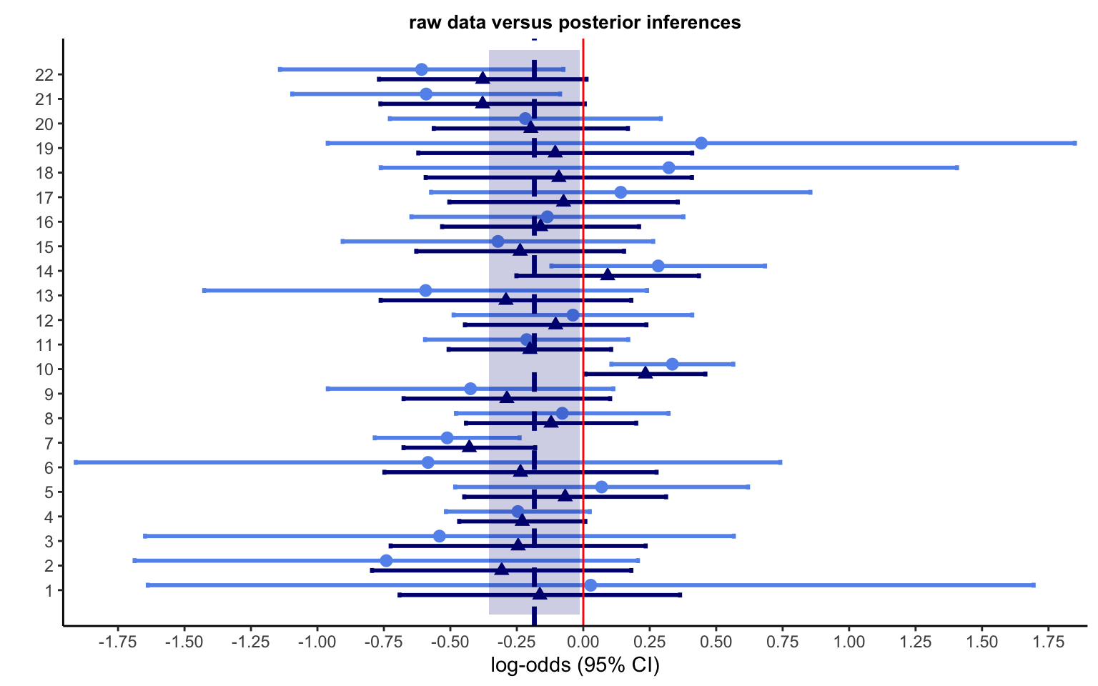
Figure 4.10 plots the data from the 22 experiments together with the posterior inferences on the true parameters (indicated by the dark blue triangles). The shaded region indicates the posterior mean and surrounding credible interval. A few other patterns stand out. The posterior means—indicated by the dark blue triangles—tend to fall closer to the meta-analytic mean than the original data means, indicated by the light blue circles. This is of course the now-familiar shrinkage to the mean of the endogenous prior at work. The posterior credible intervals are quite a bit narrower than the intervals in the data, which is also expected. Of course, meta-analysis is not always this simple. Below, we will see a case with a more complex structure.
A frequent problem in meta-analysis is that some of the statistical information needed to conduct the analysis cannot be recovered from the original papers. This mostly (but not necessarily only) concerns statistical information that would allow one to infer the standard errors surrounding the estimates of the effects of interest. Dropping such estimates risks biasing the analysis, or at the very least leads to the loss of valuable information. The good news is that one does not have to drop such observations. If one can reasonably assume that the information is missing at random—i.e. that it is not studies with particular results that would omit this information—then we can impute the missing information within the statistical code used to conduct the analysis.
I will illustrate how one can approach that problem using a set of estimates of prospect theory parameters. In the data I use below, I will focus on some complete observations of parameters for gains, including a utility curvature parameter, a likelihood-sensitivity parameter, and a pessimism parameter. This data does of course NOT encompass the universe of all estimates, so that one ought to be careful to interpret too much into the results of the analysis. It will, however, do fine as an example to develop some more advanced code for meta-analysis.
Let us assume we want to analyze the likelihood-sensitivity parameter, called sens in the data. Let us set aside for now the fact that this parameter has been obtained from different functional forms and measurements, which questions the exchangeability principle. We could now simply use the code from above to analyze this model, perhaps substituting sens for lo in the data, and designating its mean by sens_hat. The problem is that, out of the 102 observations, 16 are missing a standard error, which was not reported in the original paper from which the estimate has been taken. Throwing out these observations is clearly undesirable. Instead, we can impute the standard errors, which will allow us to keep the observations in the meta-analysis. This can be done using the following model:
data{
    int<lower=1> N;
    vector[N] sens;

//  additional elements for imputation
    int<lower=0> N_obs; // number of observed SEs
    int<lower=0> N_mis; // number of missing SEs

//indices for imputation, and observed standard errors:
    array[N_obs] int<lower = 1,upper=N> ii_obs; // index of observed values
    array[N_mis] int<lower = 1,upper=N> ii_mis; // index of missing values
    array[N_obs] real<lower=0,upper=N> se_obs; // observed SEs entered as data

//design matrix used for imputation
    int<lower=0> K; //dimension of the design matrix
    matrix[N,K] x; // design matrix to impute SEs
}
parameters{
    vector<lower=0>[N] sens_hat;
    real<lower=0> mu;
    real<lower=0> sigma;
//
    array[N_mis] real<lower=0> se_mis;
    real<lower=0> sd_se;
    vector[K] beta;
}
// compose array of SEs
transformed parameters{
    array[N] real<lower=0> se;
    se[ii_obs] = se_obs;
    se[ii_mis] = se_mis;
}
model{
//priors:
    sigma ~ cauchy( 0 , 5 );
    mu ~ normal( 1 , 5 );
    sd_se ~ normal(0 , 5);
    beta ~ normal( 0 , 5);

//imputation model
    se ~ normal( x * beta, sd_se);

//hierarchical model:
    sens ~ normal( sens_hat , se );
    sens_hat ~ normal( mu , sigma );
}
The model is best examined from the bottom up. The last two lines implement a standard meta-analysis model like seen above. The imputation model is new: it comprises a vector of standard errors, se, that is modelled as being normally distributed, with a standard deviation sd_se to be estimated, and a regression x * beta. The key to understanding the model is to examine the vector se. This vector is composed in the newly added transformed parameters block. This reveals how this vector of size N is composed of the actual data points in se_obs, which are imported as data, and a vector of variables se_mis, created in the parameters block. This way of proceeding thus reveals that the vector se is made up of some data points and some variables. The indices ii_obsand ii_mis thereby ensure the data points and variables are entered into the correct positions, i.e. corresponding to the existing and missing data on SEs, respectively. The new line in the model block thus achieves 2 things at once: 1) it uses the existing observations of the SEs to obtain the regression coefficients in beta; and 2) it simultaneously uses these coefficients and the data in the design matrix x to simulate data points for the missing observations. These are our imputed SEs. NOTE: this will of course only work as long as the data in x are available for ALL observations.
The model is thus ready to run. Care, however, needs to be taken in creating the indices and data vectors to be sent to the programme. We start by examining which variables are predictive of the SEs. It turns out that the encoded sensitivity parameter itself does a pretty good job of that by itself, capturing 27% of the variance. We then organize the values and create a unique index. Now we are ready to run the programme:
d <- read_csv("data/data_example_meta.csv",show_col_types = FALSE)
d %>% summarize(missing = sum(is.na(sens_se)))

# explore predictors of SEs
summary( lm(sens_se ~ sens,data=d) )

# create indices for missing values
d <- d %>%   mutate(obs_na = ifelse(is.na(sens_se) , 1 , 0)) %>%
             arrange(desc(obs_na)) %>%
             select(sens,sens_se,obs_na) %>%
             mutate(index = row_number())

# create data subsets for observed a missing SEs
do <- d %>% filter(!is.na(sens_se))
dm <- d %>% filter(is.na(sens_se))

# create design matrix for all data
x <- model.matrix(data = d , ~ sens)

# data to send to Stan
stanD <- list(N = nrow(d),
              K = ncol(x),
              N_obs = nrow(do),
              N_mis = nrow(dm),
              ii_obs = do$index,
              ii_mis = dm$index,
              sens = d$sens,
              se_obs = do$sens_se,
              x = x)

# execute model
ma <- cmdstan_model("stancode/meta_imp.stan")

# launch estimation
est <- ma$sample(
  data = stanD,
  seed = 123,
  chains = 4,
  parallel_chains = 4,
  refresh=200,
  init=0,
  adapt_delta = 0.999,
  max_treedepth = 15,
  iter_warmup = 1000,
  iter_sampling = 1000,
  show_messages = TRUE,
  diagnostics = c("divergences", "treedepth", "ebfmi")
)

est$print(c("mu","sigma", "beta","se_mis"), digits = 3,
          "mean", SE = "sd", "rhat", ~quantile(., probs = c(0.025, 0.975)) ,
           max_rows=20)
Even though we have forced convergence statistics, using a rather extreme adapt_delta = 0.999 and thereby slowing down convergence, we get about 2% of divergent iterations. We should thus not trust the results. Instead, we can try and improve the performance of the model by decentralizing some or all of its parameters. Let us start by decentralizing the estimated latent parameters sens_hat. To do that, we create a new vector of parameters sens_hat_z and add it in the parameter block. We then use the following transformed parameters and model blocks:
transformed parameters {
    array[N] real<lower=0> se;
    vector[N] sens_hat;

    // Compose array of SEs
    se[ii_obs] = se_obs;
    se[ii_mis] = se_mis;

  // Recenter sens_hat using decentralized parameters
    sens_hat = mu + sigma * sens_hat_z;
}
model {
    // Priors
    sigma ~ cauchy(0, 5);
    mu ~ normal(1, 5);
    sd_se ~ normal(0, 5);
    beta ~ normal(0, 5);

    //prior for sens_hat_raw
    sens_hat_z ~ std_normal( );

    // Imputation model
    se ~ normal(x * beta, sd_se);

    // measurement error model
    sens ~ normal(sens_hat, se);
}
Let us look at the bottom line of the model first, where we now include the measurement error part of the hierarchical model only. The part pertaining to the distribution of the latent parameters is shifted to the end of the transformed parameters block. Here, we now define the latent variables sens_hat as being made up of the aggregate mean, mu, plus the rescaled parameters sens_hat_z, multiplied by the standard deviation of the aggregate distribution. This means that sens_hat_z takes the form of z-scores of the sens_hat parameters, which is reflected in the standard normal distribution we give to the prior, which holds by definition. The following code estimates the model:
# execute model
ma <- cmdstan_model("stancode/meta_imp_dec.stan")

# launch estimation
est <- ma$sample(
  data = stanD,
  seed = 123,
  chains = 4,
  parallel_chains = 4,
  refresh=200,
  init=0,
  adapt_delta = 0.999,
  max_treedepth = 15,
  iter_warmup = 1000,
  iter_sampling = 1000,
  show_messages = TRUE,
  diagnostics = c("divergences", "treedepth", "ebfmi")
)


est$save_object(file="stanoutput/meta_imp_dec.Rds")
The model now converges almost twice as quickly, and the divergences almost completely disappear. Arguably, a model decentralizing the imputation model will work even better. However, this is good enough for now, and I thus leave that even more efficient model as an exercise. The figure below shows the imputed standard errors next to the observed ones, and plotted against the observed likelihood-sensitivity parameter. The imputed means of the standard errors follow the trend in the observed variables, as we should expect based on the imputation model. Importantly, however, while the observed SEs are treated as sure quantities, the imputed SEs have some uncertainty surrounding them, indicated by the plotted 95% credible intervals. The model will take this additional uncertainty into account, so that observed and imputed data enter with different weights.
# import data
d <- read_csv("data/data_example_meta.csv",show_col_types = FALSE)

# create indices for missing values
d <- d %>%   mutate(obs_na = ifelse(is.na(sens_se) , 1 , 0)) %>%
             arrange(desc(obs_na)) %>%
             select(sens,sens_se,obs_na) %>%
             mutate(index = row_number())

# create data subsets for observed a missing SEs
do <- d %>% filter(!is.na(sens_se))
dm <- d %>% filter(is.na(sens_se))

# import estimates
est <- readRDS(file="stanoutput/meta_imp_dec.Rds")

zz <- est$summary(variables = c("se_mis"), "mean", "sd")
z <- zz %>% separate(variable,c("[","]")) %>%
            rename(index = "]" , se = mean) %>%
            mutate(index = as.integer(index))

ggplot() +
  geom_point(aes(x=do$sens,y=do$sens_se), color="blue") +
  geom_point(aes(x=dm$sens,y=z$se), color="orange") +
  geom_errorbar(aes(x = dm$sens, ymin = z$se - z$sd, ymax = z$se + z$sd), color = "orange", width = 0.01) +
  labs(x="likelihood sensitivity (observed)", y= "standard error, observed (blue) and imputed (orange)")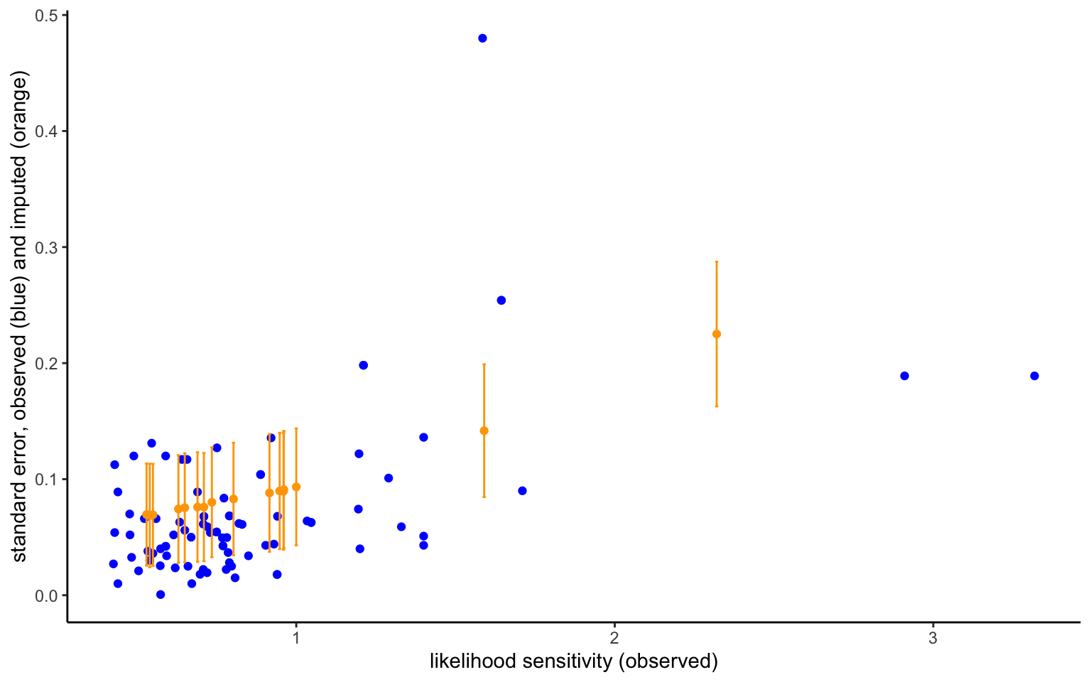
One of the goals of meta-analysis is usually to explore the correlates of the differences in effects between studies, at least in cases where those correlates are observed or can be encoded, and where there is reason to believe that such differences exist. This will not only allow one to uncover correlates, but also to discuss the degree to which they explain the between-study variance. Even if this is not the goal of your analysis, a meta-analysis such as in the examples above is of questionable solidity because it violates the exchangeability principle: at the very least, we ought to control for the functional form of the weighting function, and for the type of measurement (aggregate vs individual mean vs individual median).
Whether the model is written in a centralized or decentralized way, such a meta-regression is easy to integrate. They ke is simply to replace the mean, mu, by a regression, z * gamma, where the design matrix z used for the meta-regression will generally be different from the matrix x, used for error imputation. In this specification, z will contain a first column of 1s that implement the constant. In fact, if z only contains that column, than gamma will be a scalar equal to mu in the previous model.
data {
    int<lower=1> N;
    vector[N] sens;

    // Additional elements for imputation
    int<lower=0> N_obs; // number of observed SEs
    int<lower=0> N_mis; // number of missing SEs

    // Indices for imputation, and observed standard errors:
    array[N_obs] int<lower=1,upper=N> ii_obs; // index of observed values
    array[N_mis] int<lower=1,upper=N> ii_mis; // index of missing values
    array[N_obs] real<lower=0> se_obs; // observed SEs entered as data

    // Design matrix used for imputation
    int<lower=0> K; // dimension of the design matrix
    matrix[N,K] x; // design matrix to impute SEs

    // Design matrix used for imputation
    int<lower=0> M; // dimension of the design matrix
    matrix[N,M] z; // design matrix to impute SEs
}
parameters {
    vector[N] sens_hat_raw; // Decentralized version of sens_hat
    real<lower=0> sigma;

    // Additional parameters for imputation
    array[N_mis] real<lower=0> se_mis;
    real<lower=0> sd_se;
    vector[K] beta;
    vector[M] gamma;
}
transformed parameters {
    array[N] real<lower=0> se;
    vector[N] sens_hat; // Recentered sens_hat

    // Compose array of SEs
    se[ii_obs] = se_obs;
    se[ii_mis] = se_mis;

    // Recenter sens_hat using decentralized parameters
    sens_hat = z * gamma + sigma * sens_hat_raw;
}
model {
    // Priors
    sigma ~ cauchy(0, 5);
    sd_se ~ normal(0, 5);
    beta ~ normal(0, 5);
    gamma ~ normal(0, 5);
    sens_hat_raw ~ std_normal( ); // Standard normal prior for decentralized parameter

    // Imputation model
    se ~ normal(x * beta, sd_se);

    // Hierarchical model
    sens ~ normal(sens_hat, se);
}
The following code executes the meta-regression:
d <- read_csv("data/data_example_meta.csv",show_col_types = FALSE)
d %>% summarize(missing = sum(is.na(sens_se)))

# explore predictors of SEs
summary( lm(sens_se ~ sens,data=d) )

# create indices for missing values
d <- d %>%   mutate(obs_na = ifelse(is.na(sens_se) , 1 , 0)) %>%
             arrange(desc(obs_na)) %>%
             mutate(index = row_number()) %>%
             mutate(prelec2 = ifelse(pwf_form=="LLO",0,1))

# create data subsets for observed a missing SEs
do <- d %>% filter(!is.na(sens_se))
dm <- d %>% filter(is.na(sens_se))

# create design matrix for imputation
x <- model.matrix(data = d , ~ sens)

# design matrix for meta-regression
z <- model.matrix(data = d , ~ prelec2)

# data to send to Stan
stanD <- list(N = nrow(d),
              K = ncol(x),
              M = ncol(z),
              N_obs = nrow(do),
              N_mis = nrow(dm),
              ii_obs = do$index,
              ii_mis = dm$index,
              sens = d$sens,
              se_obs = do$sens_se,
              x = x,
              z = z)

# execute model
ma <- cmdstan_model("stancode/meta_imp_reg.stan")

# launch estimation
est <- ma$sample(
  data = stanD,
  seed = 123,
  chains = 4,
  parallel_chains = 4,
  refresh=200,
  init=0,
  adapt_delta = 0.999,
  max_treedepth = 15,
  iter_warmup = 1000,
  iter_sampling = 1000,
  show_messages = TRUE,
  diagnostics = c("divergences", "treedepth", "ebfmi")
)

est$print(c("gamma","sigma", "beta","se_mis"), digits = 3,
          "mean", SE = "sd", "rhat", ~quantile(., probs = c(0.025, 0.975)) ,
max_rows=20) The code above provides the fundamental building blocks for meta-analysis. That being said, how to build the model exactly will depend on the actual questions of interest. For instance, while at the lowest level we are forced to assume a normal distribution, a different type of distribution may well be called for at the aggregate level (e.g., a lognormal form usually fits better for the types of constrained parameters considered above). One may further want to explicitly model dependency between different studies stemming from the same paper, either by additional hierarchical levels, or by cross-classification. And in the specific case above, one may want to analyze the three parameters jointly, rather than in isolation. All of this is fairly straightforward to include in Stan, and you should now have the tools to do so yourself.
Above, we have seen a way to integrate regressions directly into the models estimating the parameters. While this is a principled way of conducting regressions, it may at times not be very practical, e.g. because your estimation takes a long time to complete, and you need to run many regressions. In such cases, one can use a two-stage procedure: by explicitly treating the parameters as quantities measured with error, one can then nevertheless avoid the fallacy of standard two-stage procedures using the parameter mean, which problematically treat estimated parameters as objectively observed quantities and throw away the information we have on our confidence in the value we estimate (conditional on the model we assume). The price to pay is that we will need to assume the posterior of the parameters to follow a normal distribution. This assumption is often good enough, and of course it can be tested if you have access to the full posteriors.
Given the tools we have explored above, building such a regression is now quite trivial. We first model the parameter we want to regress—let us call it generically theta—as a quantity measured with uncertainty, so that theta ~ normal(theta_hat, se);, just like done above for meta-analysis. Except that now, thetais an estimated parameter and se its associated standard deviation of the posterior. The rest proceeds like the meta-regression discussed above, which I here implement using a robust Student-t distribution with 3 degrees of freedom:
data {
    int<lower=1> N;
    vector[N] theta;
    vector[N] se;

   // Design matrix used for regression
    int<lower=0> K; // dimension of the design matrix
    matrix[N,K] x; // design matrix to impute SEs
}
parameters {
    vector[N] theta_hat;
    real<lower=0> sigma;
    vector[K] beta;
}
model {
    // Priors
    sigma ~ normal(0, 2);
    beta ~ normal(0, 2);

    // Measurement error model
    theta ~ normal(theta_hat, se);

    // Regression model:
    theta_hat ~ student_t(3 , x * beta  , sigma );
}
For simplicity, let us use again the estimates from Bruhin, Fehr-Duda, and Epper (2010) that we have examined above, and look at the same regression for the likelihood-sensitivity parameter.
hc <- readRDS(file="stanoutput/RR_CH6_RDU.Rds")

zz <- hc$summary(variables = c("rho","gamma","delta","sigma"), "mean" , "sd")
zc <- zz %>% separate(variable,c("[","]")) %>%
            rename( var = `[`) %>% rename(id = `]`) %>%
            pivot_wider(names_from = var , values_from = c(mean,sd)) %>%
            rename(rho = mean_rho , gamma = mean_gamma , delta = mean_delta , sigma = mean_sigma) %>%
            mutate(id = as.numeric(id))

#
d <- read_csv("data/data_RR_ch06.csv")

dg <- d %>% filter(z1 > 0) %>%
            mutate(high = z1) %>%
            mutate(low = z2) %>%
            mutate(prob = p1) %>%
            group_by(id) %>%
            mutate(id = cur_group_id()) %>%
            ungroup()

di <- dg %>% group_by(id) %>%
             filter(row_number()==1) %>%
             ungroup()

z <- left_join(di,zc,by="id")

# design matrix
x <- model.matrix( ~ 1 + female + semester,z)


# data to send to Stan
stanD <- list(N = nrow(z),
              theta = z$gamma,
              se = z$sd_gamma,
              x = x,
              K = ncol(x))

# execute model
ma <- cmdstan_model("stancode/reg2s_mem.stan")

# launch estimation
est <- ma$sample(
  data = stanD,
  seed = 123,
  chains = 4,
  parallel_chains = 4,
  refresh=200,
  init=0,
  adapt_delta = 0.85,
  max_treedepth = 12,
  iter_warmup = 1000,
  iter_sampling = 1000,
  show_messages = TRUE,
  diagnostics = c("divergences", "treedepth", "ebfmi")
)

est$save_object(file="stanoutput/reg2s_mem.Rds")est <- readRDS("stanoutput/reg2s_mem.Rds")
est$print(c("beta","sigma"), digits = 3,
"mean", SE = "sd", "rhat", ~quantile(., probs = c(0.025, 0.975)) ,
max_rows=20) variable mean SE rhat 2.5% 97.5%
beta[1] 0.529 0.035 1.002 0.461 0.597
beta[2] -0.111 0.036 1.003 -0.182 -0.040
beta[3] 0.003 0.007 1.001 -0.011 0.016
sigma 0.185 0.013 1.003 0.161 0.213We again find a negative effect of the gender dummy. The quantitative effect is indeed arbitrarily close to the one we documented above, while taking the full parameter uncertainty into account and estimating the regression jointly with the model parameters. In general, however, this approach will only work well as long as errors are at least approximatley normally distributed around the estimated parameters—something that is up to you to check when you are estimating the parameters.
We have so far seen mostly models with 2 hierarchical levels—subjects drawn from a common group may be the classical example. In many cases, however, it will be desirable to construct more complex hierarchies than the ones we have examined so far. For instance, in the 30 country model a meaningful model would treat subjects as being drawn from a national distribution, and countries as being drawn from a global distribution, thus resulting in 3 hierarchical levels. In other cases, some observations may belong to two different categories along different dimensions. Stan is very flexible in allowing for multiple hierarchical levels and cross-classification, whereby observations may at the same time belong to different categories. Such more complex models are essential when e.g. modelling stratified sampling designs. Here, I discuss how to implement such complex hierarchies for the nonlinear models we have examined.
Let us start from the simple random intercept model we discussed above. I will now use the Ethiopian data of Vieider et al. (2018), since the smaller size of the data will ensure that the example code converges quickly. As a reminder, the simple, 2-level model with random intercepts takes the following form, where I now use n for the individual-level intercepts, and s for the slope measuring likelihood-dependence, which is assumed to be the same for everybody. The line n ~ normal(mu, tau); uses vector notation to model the individual-level intercepts as drawn from an aggregate distribution with mean mu and standard deviation tau.
data{
int<lower=0> N;
int<lower=0> Nid;
vector[N] ce;
vector[N] p;
array[N] int id;
}
parameters{
real mu;
real s;
real<lower=0> sigma;
real<lower=0> tau;
vector[Nid] n;
}
model{
// hyperpriors for aggregate parameters
mu ~ std_normal( );
s ~ normal( 1 , 1 );
sigma ~ normal( 0.2 , 2 );
tau ~ normal( 0.2 , 2 );

//distribution of intercepts
n ~ normal(mu, tau);

//regression model with individual-level intercept
ce ~ normal( n[id] + s * p , sigma  ) ;
}
The following code runs the model and estimates the parameters:
d <- read_csv("data/data_ETH.csv")
d <- d %>% group_by(subject) %>%
           mutate(id = cur_group_id()) %>%
           ungroup()

# creates data to send to Stan
stanD <- list(N = nrow(d),
              ce = d$equivalent/d$high,
              p = d$probability,
              Nid = max(d$id),
              id = d$id)


# compile the Stan programme:
sr <- cmdstan_model("stancode/ri_ETH.stan")

# run the programme:
nm <- sr$sample(
  data = stanD,
  seed = 123,
  chains = 4,
  parallel_chains = 4,
  refresh=200,
  init=0,
  show_messages = TRUE,
  diagnostics = c("divergences", "treedepth", "ebfmi")
)

print(nm, c("mu","s","sigma","tau","n"),digits = 3)
Assume we are interested in risk attitudes across the Ethiopian rural highlands (the study population underlying the data). We might be tempted to use (some indices based on) the mean mu and the aggregate slope s to characterize such preferences. However, the model used above would introduce bias into our estimation results, simply because we are ignoring the study design. Indeed the study used a stratified design, whereby Woredas (Ethiopian administrative districts) were randomly selected from the study region. Subjects were subsequently randomly selected from these Woredas. To be able to infer the attitudes of a representative agent, we will thus need to explicitly model this sampling design (cfr. BDM3 for details).
The simplest way of introducing the additional hierarchical level is to proceed exactly like above. In particular, we will now want the individual-level intercepts n to have a Woreda-level mean w, which values corresponding to the means in the 21 Woredas in the data; and we will then distribute the Woreda-level means as being drawn from an aggregate distribution. To make sure that the dimensions agree at the different levels, it is further convenient to introduce two loops to the code:
data {
  int<lower=0> N;
  int<lower=0> Nid;
  int<lower=0> Nw;
  vector[N] ce;
  vector[N] p;
  array[N] int id;
  array[N] int wid;
}
parameters {
  real mu;
  real s;
  real<lower=0> sigma;
  real<lower=0> xi;
  real<lower=0> tau;
  vector[Nid] n;
  vector[Nw] w;
}
model {
  // hyperpriors for aggregate parameters
  mu ~ std_normal();
  s ~ normal(1, 1);
  sigma ~ normal(0.2, 2);
  tau ~ normal(0.2, 2);
  xi ~ normal(0.2, 2);

  // distribution of Woreda-level intercepts
  w ~ normal(mu, tau);

  // distribution of intercepts at the Woreda level
  for (n in 1:Nid)
    n[n] ~ normal(w[wid[id[n]]], xi);

  // regression model with individual-level intercept
  for (i in 1:N)
    ce[i] ~ normal(n[id[i]] + s * p[i], sigma);
}d <- read_csv("data/data_ETH.csv")
d <- d %>% group_by(subject) %>%
mutate(id = cur_group_id()) %>%
ungroup() %>%
group_by(Woreda) %>%
mutate(wid = cur_group_id()) %>%
ungroup()
# creates data to send to Stan
stanD <- list(N = nrow(d),
ce = d$equivalent/d$high,
p = d$probability,
Nid = max(d$id),
id = d$id,
Nw = max(d$wid),
wid = d$wid)
# compile the Stan programme:
sr <- cmdstan_model("stancode/ri_ETH2.stan")
# run the programme:
nm <- sr$sample(
data = stanD,
seed = 123,
chains = 4,
parallel_chains = 4,
refresh=200,
init=0,
adapt_delta = 0.99,
max_treedepth = 15,
show_messages = TRUE,
diagnostics = c("divergences", "treedepth", "ebfmi")
)
print(nm, c("mu","s","sigma","tau","n"),digits = 3)This model works. However, it has become quite slow. I further had to crank up the adapt_delta metric to .99 to get reasonably convergence, and even then, a number of divergence remains—too many to look the other way. The key, as so often in Stan, is to decentralize the parameters. This is done below in the line n = mu_w + w[wid[id[1:Nid]]] + xi * n_z;, which moves the estimation of the individual-level estimates to the transformed data block, and defines them in function of the stndardized parameters in n_z, which follow a standard normal distribution as usual. There are two additional elements I would like to point out. The first is the indexing in w[wid[id[1:Nid]]]: This tells Stan that a particular id is associated to a particular wid, and that the id ranges from 1:Nid (Stan would otherwise attempt to include all observations, resulting in paradoxical results in the estimates w parameters). The second thing to note is that I have reverted from the loop in the previous version to the vectorized version of the likelihood, ce ~ normal( n[id] + s * p , sigma ) ;. Both will work, but this simple change brings the running time from 10 to 3 minutes on my laptop. Finally, one could, of course, also decentralize the Woreda-level intercepts in w. In this particular case at least, that however makes things worse rather than further improving the model.
data {
  int<lower=0> N;           // Number of observations
  int<lower=0> Nid;         // Number of individual-level units
  int<lower=0> Nw;          // Number of Woreda-level units
  vector[N] ce;             // Outcome variable
  vector[N] p;              // Predictor variable
  array[N] int id;          // Individual-level indices
  array[N] int wid;         // Woreda-level indices
}
parameters {
  real mu_w;                // Global mean for Woreda-level intercepts
  real<lower=0> tau_w;      // Between-Woreda variance
  real<lower=0> sigma;      // Observation-level noise
  real<lower=0> xi;         // Between-individual variance within Woredas
  vector[Nw] w;             // Woreda-level intercepts
  vector[Nid] n_z;        // Individual-level deviations (standard normal)
  real s;                   // Slope coefficient for the predictor
}
transformed parameters {
  vector[Nid] n;            // Individual-level intercepts
  n = mu_w + w[wid[id[1:Nid]]] + xi * n_z;
}
model {
  // Priors
  mu_w ~ std_normal();                // Prior on global mean
  tau_w ~ normal(0, 1);               // Prior on Woreda-level variance
  xi ~ normal(0, 1);                  // Prior on individual-level variance
  sigma ~ normal(0.2, 2);             // Prior on noise
  s ~ normal(1, 1);                   // Prior on slope

  // Woreda-level effects
  w ~ normal(0, tau_w);               // Woreda-level intercepts

  // Individual-level deviations
  n_z ~ std_normal();               // Raw individual deviations

  // Likelihood
  ce ~ normal( n[id] + s * p , sigma  ) ;
}d <- read_csv("data/data_ETH.csv")
d <- d %>% group_by(subject) %>%
mutate(id = cur_group_id()) %>%
ungroup() %>%
group_by(Woreda) %>%
mutate(wid = cur_group_id()) %>%
ungroup()
# creates data to send to Stan
stanD <- list(N = nrow(d),
ce = d$equivalent/d$high,
p = d$probability,
Nid = max(d$id),
id = d$id,
Nw = max(d$wid),
wid = d$wid)
# compile the Stan programme:
sr <- cmdstan_model("stancode/ri_ETH2_dec.stan")
# run the programme:
nm2 <- sr$sample(
data = stanD,
seed = 123,
chains = 4,
parallel_chains = 4,
refresh=200,
init=0,
adapt_delta = 0.95,
max_treedepth = 18,
show_messages = TRUE,
diagnostics = c("divergences", "treedepth", "ebfmi")
)
print(nm2, c("n","s","sigma"),digits = 3)Of course, nothing stops us from expanding the model to including a random slope as well. The likelihood then becomes ce ~ normal( n[id] + s[id] .* p , sigma[id] ) ;, where .* implements the dot product. This ensures compatibility between the different dimensions. In addition to that, all that is required is to add a second line s = mu_s + w_s[wid[id[1:Nid]]] + xi_s * s_raw; in the transformed parameters block (and of course to create the new variables and to give them priors). Nevertheless, it may be desirable to collect these two lines using matrix notation, since that will allow us to add a covariance matrix. The transformed parameters block then becomes as follows, where the loop is being used mainly for coding transparency:
```{stan, output.var="model_test.stan", eval = FALSE, tidy = FALSE} transformed parameters { array[Nid] vector[2] pars; vector[Nid] n; vector[Nid] s; for (j in 1:Nid){ pars[j] = means + W[wid[id[j]]] + diag_pre_multiply(xi, L_omega) * Z[j]; n[j] = pars[j,1] ; s[j] = pars[j,2] ; } }
The following code runs the model:
d <- read_csv("data/data_ETH.csv")
d <- d %>% group_by(subject) %>%
           mutate(id = cur_group_id()) %>%
           ungroup() %>%
           group_by(Woreda) %>%
           mutate(wid = cur_group_id()) %>%
           ungroup()

# creates data to send to Stan
stanD <- list(N = nrow(d),
              ce = d$equivalent/d$high,
              p = d$probability,
              Nid = max(d$id),
              id = d$id,
              Nw = max(d$wid),
              wid = d$wid)


# compile the Stan programme:
sr <- cmdstan_model("stancode/rirs_ETH2_covar.stan")

# run the programme:
nm2 <- sr$sample(
  data = stanD,
  seed = 123,
  chains = 4,
  parallel_chains = 4,
  refresh=200,
  init=0,
  adapt_delta = 0.9,
  max_treedepth = 15,
  show_messages = TRUE,
  diagnostics = c("divergences", "treedepth", "ebfmi")
)

print(nm2, c("W","s","n"),digits = 3)

nm2$save_object(file="stanoutput/rirs_ETH2_dec.Rds")Note that there is also a different possibility to efficiently introduce the additional level. It involves defining the intercept at the lowest level, call it n_obs, which will have N dimensions. Notice that we now have a different intercept for each data point or certainty equivalent in this case. This variable can then be defined in the transformed parameters block while looping through all observations. We then use n_z to obtain decentralized individual-level intercepts. Since we are looping through all observations, it is further straightforward to add Woreda-level effects (or indeed regression coefficients, or effects at any other level that may interest you). If you are interested in the individual-level intercepts, you may want to recover them by adding an individual-level loop in the generated quantities block. Notice, however, that this is not quite the same model: you are de facto defining a “random preference model”, where preference parameters are allowed to change for each single choice, though they are constrained by having an individual-level mean. Indeed, the parameters in the likelihood, ce ~ normal(n_obs + s_obs * p, sigma);, are now defined at the level of the observation.
data {
  int<lower=0> N;           // Number of observations
  int<lower=0> Nid;         // Number of individual-level units
  int<lower=0> Nw;          // Number of Woreda-level units
  vector[N] ce;             // Outcome variable
  vector[N] p;              // Predictor variable
  array[N] int id;          // Individual-level indices
  array[N] int wid;         // Woreda-level indices
}
parameters {
  real mu;                // Global mean for Woreda-level intercepts
  real<lower=0> tau;      // Between-Woreda variance
  real<lower=0> sigma;      // Observation-level noise
  real<lower=0> xi;         // Between-individual variance within Woredas
  vector[Nw] w;             // Woreda-level intercepts
  vector[Nid] n_z;        // Individual-level deviations (standard normal)
  real s;                   // Slope coefficient for the predictor
}
transformed parameters {
  vector[N] n_obs;              // Individual-level intercepts for each observation
  for (i in 1:N)
    n_obs[i] = mu + w[wid[i]] + xi * n_z[id[i]];
}
model {
  // Priors
  mu_w ~ std_normal();                // Prior on global mean
  tau_w ~ normal(0, 1);               // Prior on Woreda-level variance
  xi ~ normal(0, 1);                  // Prior on individual-level variance
  sigma ~ normal(0.2, 2);             // Prior on noise
  s ~ normal(1, 1);                   // Prior on slope

  // Woreda-level effects
  w ~ normal(0, tau);               // Woreda-level intercepts

  // Individual-level deviations
  n_z ~ std_normal();               // Raw individual deviations

  // Likelihood
  ce ~ normal(n_obs + s_obs * p, sigma);      // Regression model
}d <- read_csv("data/data_ETH.csv")
d <- d %>% group_by(subject) %>%
mutate(id = cur_group_id()) %>%
ungroup() %>%
group_by(Woreda) %>%
mutate(wid = cur_group_id()) %>%
ungroup()
# creates data to send to Stan
stanD <- list(N = nrow(d),
ce = d$equivalent/d$high,
p = d$probability,
Nid = max(d$id),
id = d$id,
Nw = max(d$wid),
wid = d$wid)
# compile the Stan programme:
sr <- cmdstan_model("stancode/rirs_ETH2_obs.stan")
# run the programme:
nm3 <- sr$sample(
data = stanD,
seed = 123,
chains = 4,
parallel_chains = 4,
refresh=200,
init=0,
adapt_delta = 0.9,
max_treedepth = 15,
show_messages = TRUE,
diagnostics = c("divergences", "treedepth", "ebfmi")
)
print(nm2, c("W","s","n"),digits = 3)
nm3$save_object(file="stanoutput/rirs_ETH2_obs.Rds")The model is more than 3 times faster to estimate than the one with the individual-level parameters only, which may seem paradoxical, given that it comprises many more parameters. This may well be a sign that it fits better, i.e. that the posterior is easier to explore. A potentially interesting question concerns the inferences we draw on the individual-level parameters. The figures below show correlations of individual-level parameters estimated in the two models. They are indeed very similar, though slightly dispersed in the observation-level model around the value in the individual-level model. The slight shift in parameters seems to stem from increased uncertainty in some parameters, which yields stronger shrinkage to the Woreda-level means. Which model you prefer depends on your substantive questions, and is for you to decide.
nm2 <- readRDS("stanoutput/rirs_ETH2_dec.Rds")
nm3 <- readRDS("stanoutput/rirs_ETH2_obs.Rds")


zz <- nm2$summary(variables = c("n","s"), "mean", "sd")
z2 <- zz %>% separate(variable,c("[","]")) %>%
            rename(index = "]",var = "[") %>%
            pivot_wider(names_from = var , values_from = c(mean,sd)) %>%
            mutate(index = as.integer(index)) %>%
            rename(n = mean_n,s = mean_s)

zz <- nm3$summary(variables = c("n","s"), "mean", "sd")
z3 <- zz %>% separate(variable,c("[","]")) %>%
            rename(index = "]",var = "[") %>%
            pivot_wider(names_from = var , values_from = c(mean,sd)) %>%
            mutate(index = as.integer(index)) %>%
            rename(no = mean_n,so = mean_s)

z <- left_join(z2,z3,by="index")


ggplot(z,aes(x=n,y=no)) +
  geom_point( color="blue") +
  geom_abline(intercept=0,slope=1) +
  labs(x="intercept, individual model", y= "intercept, observational model")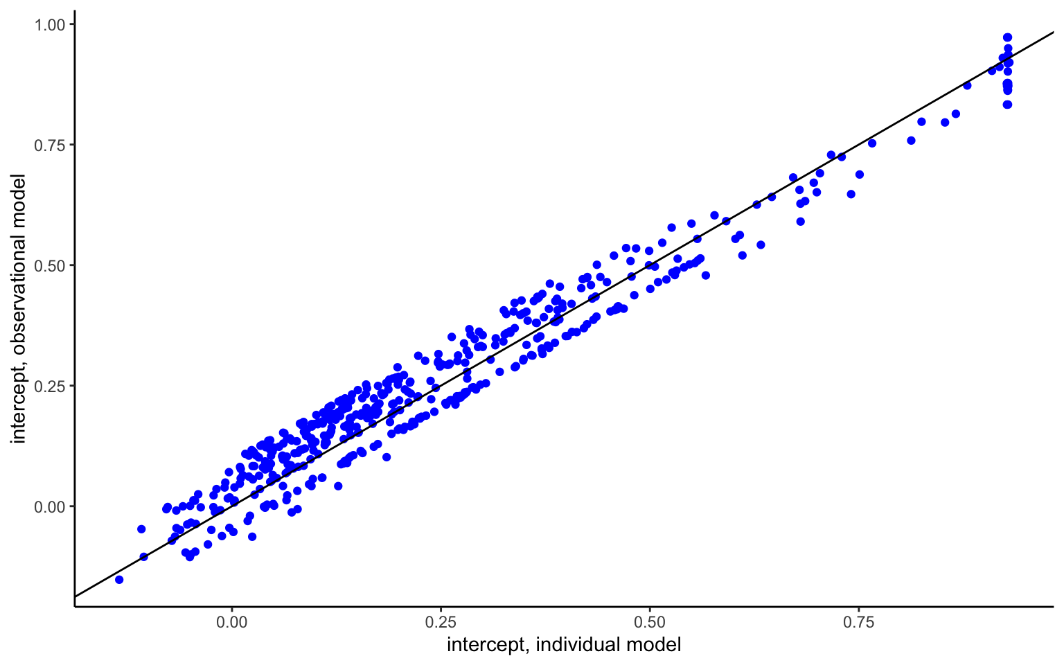
This is the end as of 03 September 2024. Stand by for additional sections to be added soon.