2  Bayesian Foundations

This chapter contains a discussion of the foundations of Bayesian statistics. I focus on simple conjugate analysis of the most common distributional families. This serves to build theoretical underpinnings that will prove invaluable in the interpretation of more complex models in later chapters. It will furthermore help in developing a thorough understanding of the relative role of the prior and the data in determining the inferences we draw. This is an extremely important exercise, since the effect of priors is something that often confuses non-Bayesians upon first impact with Bayesian techniques. It is, however, important to keep in mind that Bayesian analysis is much more about taking uncertainty seriously than it is about priors. Exploring these issues using simulated data and sequential updating will allow us to paint a precise picture of how exactly the influence of the prior vanes as subsequent data points are added. Beyond the examples provided, it is always a good idea to look at the underlying code, and to tweak any parameters of interest to see the effect that may have on the posterior inferences!

2.1 Bayes’ equation

Bayes’ equation is likely the single most important equation in all of statistics, if not life and nature in general. The fundamental idea is simple. Say we want to make an inference on the likelihood of a hypothesis, designated by \(h\). We have some data that might be informative on this issue, call them \(d\). What we want to find out is the probability that the hypothesis is true or false, given the data (and yes, the data are truly given in this context). This is a hard problem to answer directly. Instead, we may want to think about an easier problem, such as what is the likelihood of the data, given the hypothesis, as done in classical statistics. This is an easier problem because in an idealized experiment we can use the hypothesis to generate a large number of simulated datasets and see how often such a newly drawn dataset will resemble the one at hand. We can then use this to answer our original query in the following way:

\[ p(h \, | \, d) = \frac{p(d \,| \, h) \, p(h)}{p(d)} \]

where \(p(d)\) is the total probability of the data, i.e. \(p(d) = \sum_i p(d \, | \, h_i) \, p(h_i)\), or \(\int p(d\, | \, h)\, p(h) \,dh\) for a continuous hypothesis space. This is called a marginal distribution in Bayesian statistics, and summing over all possible cases to eliminate the conditionality statements is thus called marginalization.

The trouble is that the denominator is difficult to calculate precisely in most situations, and may not allow a closed form solution at all. We thus often see the equation written in the following way:

\[ p(h \, | \, d) \propto p(d \, | \, h) \, p(h), \] where \(\propto\) indicates proportionality and is read as is proportional to. That is, we can usually simulate the posterior distribution by the above expression, without calculating \(p(d)\) precisely. This is a legitimate strategy, inasmuch as the marginal density \(p(d)\) does not contain the hypothesis, so that it can be considered a constant. This also means, however, that no analytic solutions will generally be possible—we will have to rely on simulations only. This is indeed why Bayesian analysis has been a minority pursuit for a long time. However, with the ever-increasing availability of fast computing and the consequent development of dedicated Bayesian statistics packages, Bayesian statistics is quickly emerging as a viable alternative to the classical, frequentist type.

Luckily, there is a way of circumventing the thorny issue of calculating the normalization constant all together: we can use conjugate priors. A conjugate prior is a prior such that the posterior distribution obtained by combining likelihood and prior will belong to the same distributional family as the prior itself. This allows us to derive analytic solutions for the posterior, and is thus extremely useful in illustrating the workings underlying Bayesian analysis. This first chapter is dedicated to developing the underlying formalism, and to showing a number of practical examples. Two distributions will prove particularly useful—distributions from the Bernoulli-Binomial-Beta family, and distributions from the Gaussian family. We will start from the former.

2.2 Beliefs about proportions

We start from the standard example of a series of data points \(x = \{x_1, … , x_n\}\), which can take the value of 1 (success) or 0 (failure). A fitting example may be that we want to estimate the proportion of trustworthy individuals in a population, and we want to obtain a probability of a random individual from the population being trustworthy. Here and in sequence, I will assume the data points to be exchangeable (equivalent to an i.i.d. assumption), unless stated otherwise.

Let us assume that you observe a single realization from the data vector, call it \(x_i\). We want to find the probability that \(x_i = 1\), call it \(p(x_i=1 \, | \,\theta) = \theta\) (the notation emphasizes that this designates the probability of the data, conditional on the parameter; the same letter is used for the variable and its concrete value in this case, since no ambiguity arises from this). Since \(0 \le \theta \le 1\), we know that \(p(x_i = 0 \, | \, \theta) = 1 - \theta\). The probability distribution will thus take the form of a Bernoulli function:

\[ p(x_i \, | \, \theta) = \theta^{x_i} \, (1-\theta)^{1 - x_i}, \] with a mean of \(\theta\) and a variance of \(\theta \, (1-\theta)\). If the observations are exchangeable as assumed here, one can see directly that the probability of the overall data takes the following form

\[ p(x \, | \, \theta) = \prod_{i=1}^N p(x_i \, | \, \theta) \] A frequentist approach to the data would consist in maximizing the likelihood of the function above, although for computational reasons in practice it is usual to maximize the logarithm of the likelihood, which has the following form:

\[\begin{align*} ln \enspace p(x \,| \, \theta) &= \sum_{i=1}^N ln \enspace p(x_i \, | \, \theta) \\ &= \sum_{i=1}^N[\, x_i \, ln(\theta) + (1-x_i) \, ln(1-\theta) \,]. \end{align*}\] Taking the derivative with respect to \(\theta\) and setting it to zero, we obtain the following maximum likelihood estimate:

\[ \theta_{ML} = \frac{1}{N}\sum_{i=1}^N x_i, \] which indicates that the maximum-likelihood estimate of the probability is simply equal to the sample mean of the observations.

Although this approach will work well with large samples, it can lead to paradoxical conclusions based on small samples. Suppose that we flip a coin 4 times, and that all of the coins come up heads, encoded as 1. The maximum likelihood estimate then predicts that all future coin flips should come up heads. This seems an extreme prediction, illustrating the overfitting maximum likelihood techniques are prone to when using small samples. Before you protest that such a small sample is absurd, stop and think about the number of observations we often have when trying to assess the preference parameters of single individuals, where the models we try to fit are typically much more complex than in the example above.

We can also get at the solution described above more directly. Let \(m\) designate the number of successes out of \(N\) trials. We can then write the likelihood of this number of successes directly according to the Binomial model:

\[\begin{align*} p(m \, | \, \theta) &= Bin(m \, | \, N,\theta) \\ &= \binom{N}{m} \, \theta^m \,(1-\theta)^{N-m}. \end{align*}\]

In classical statistics, we would simply calculate this statistic from the sample, and possibly determine whether the conditions, such as the size of the sample, are such as to guarantee an unbiased estimate (though this is often neglected in practice). In the Bayesian setup we are interested in, however, the parameter \(\theta\) is an uncertain quantity, while the data are considered given. We could then interpret the \(\theta\) estimate obtained based on the above likelihood as a random draw from a distribution of possible estimates. As hinted at above, this will be especially advantageous when we are working with small datasets, potentially just one observation at the time.

We can thus specify a prior distribution that contains all kinds of knowledge we may have about the distribution of the parameter \(\theta\), simply written as \(p(\theta)\). While in theory we could use any functional form, in practice it is often convenient to work with so-called conjugate distributions, i.e. functional forms which combined with the likelihood will yield a posterior that exhibits the same functional form as the prior. To do this, we can rewrite the likelihood above purely as a function of \(\theta\) (we can do this because the remainder of the equation purely serves to normalize the density to 1, which we can also do ex post):

\[ p(x \, | \, \theta) \propto \theta^m \,(1-\theta)^{N-m}. \] We now want a prior density that has the same form, which so happens to be the Beta distribution:

\[ p(\theta) \propto \theta^{\alpha - 1}(1-\theta)^{\beta - 1}, \] where I have again omitted the normalization constant since it is not important for our purposes.

To obtain the posterior distribution, we will need to multiply the likelihood with the prior. The posterior we obtain will again follow the same parametric form. Combining the likelihood and prior above, we can easily get the posterior distribution:

\[\begin{align*} p(\theta \, | \, x) &\propto p(x \, | \, \theta) \, p(\theta) \\ &\propto \theta^m \, (1-\theta)^{N-m} \, \theta^{\alpha - 1} \, (1-\theta)^{\beta - 1} \\ &\propto Beta(\theta \, | \, \alpha + m \, , \, \beta + N - m). \end{align*}\] From this, we may obtain the posterior mean and variance as follows:

\[\begin{align*} E(\theta \, | \,x) &= \frac{\alpha + m}{\alpha + \beta + N} \\ var(\theta|x) &= \frac{(\alpha + m)(\beta + N - m)}{(\alpha + \beta + N)^2(\alpha + \beta + N + 1)} \\ &=\frac{E(\theta|x) \, [1 - E(\theta \, | \,x)]}{\alpha + \beta + N + 1}. \end{align*}\]

These equations serve to illustrate some fundamental properties of Bayesian analysis. For instance, as \(m\) and \(N\) become large for fixed parameters of the prior, the posterior expectation will converge to the sampling expectation, \(\lim_{N \rightarrow \infty}E(\theta \, | \, x, \alpha , \beta) = \frac{m}{N}\). Equivalently, the variance will approach zero as \(N\) gets large, so that \(var(\theta \, | \, x) \approx \frac{1}{N}\frac{m}{N} \, (1-\frac{m}{N})\). That is, in the limit the prior has no influence over the posterior distribution. We can also easily see how new observations of successes or failures simply go to augment the parameters of the Beta distribution. This is especially useful in sequential updating, which I discuss next.

2.2.1 Sequential updating

In many applications, it will be interesting to update the prior sequentially as new information comes along. The posterior distribution derived from updating the prior with a new observation will then itself become the prior for the subsequent observation. The updating equations of the two parameters will simply take the following form:

\[\begin{align*} \alpha_{i+1} &= \alpha_i + x_i \\ \beta_{i+1} &= \beta_i + (1 - x_i), \end{align*}\] where \(\alpha_i\) and \(\beta_i\) are the parameters of the prior for the observation in period/round \(i\), and the updated parameters indexed by \(i+1\) are the posterior parameters from the perspective of period \(i\), as well as the prior parameters from the perspective of period \(i+1\), i.e. for the subsequent update with \(x_{i+1}\). (The result obtains trivially by multiplying a Bernoulli likelihood with a Beta prior).

We can use this function to sequentially update our Beta prior. It will be helpful to illustrate this with a dataset of binary choices. Let us assume that we present a subject with choices between different sure amounts \(c\) and a lottery paying \(y\) with probability 0.5, or else 0. We know that the sure amounts \(c\) are equally spaced between \(y\) and 0, and that there is an equal number of sure amounts below and above the expected value \(py\). The simplest way of discovering the preferences of the decision maker will then be to count the number of choices for the sure amount, indicated by \(x_i = 1\).

obs <- rbernoulli(n=50,p=0.71) 
x <- append(obs,0,0)

alpha <- 2 
beta <- 2

for(i in 2:51){ alpha[i] <- alpha[i-1] + x[i] 
                beta[i] <- beta[i-1] + (1 - x[i]) }

ggplot(data = data.frame(x = c(0, 1)), aes(x=x)) + 
  stat_function(fun = dbeta, n = 101, args = list(shape1 = alpha[1], shape2 = beta[1]), linewidth=1.5,aes(colour="0 obs. (prior)")) + 
  stat_function(fun = dbeta, n = 101, args = list(shape1 = alpha[2], shape2 = beta[2]), aes(colour="1 obs."),linewidth=1.5) + 
  stat_function(fun = dbeta, n = 101, args = list(shape1 = alpha[11], shape2 = beta[11]), aes(colour="10 obs"),linewidth=1.5) + 
  stat_function(fun = dbeta, n = 101, args = list(shape1 = alpha[51], shape2 = beta[51]), aes(colour="50 obs"),linewidth=1.5) + 
  geom_vline(xintercept=mean(obs), aes(colour="red"), linetype="dashed") + ylab("") + scale_y_continuous(breaks = NULL) + 
  xlab("proportion of safe choices") + 
  scale_colour_manual("Legend", values = c("black","darkgoldenrod", "chocolate4", "darkolivegreen4")) + 
  theme(legend.position = c(0.2, 0.75))

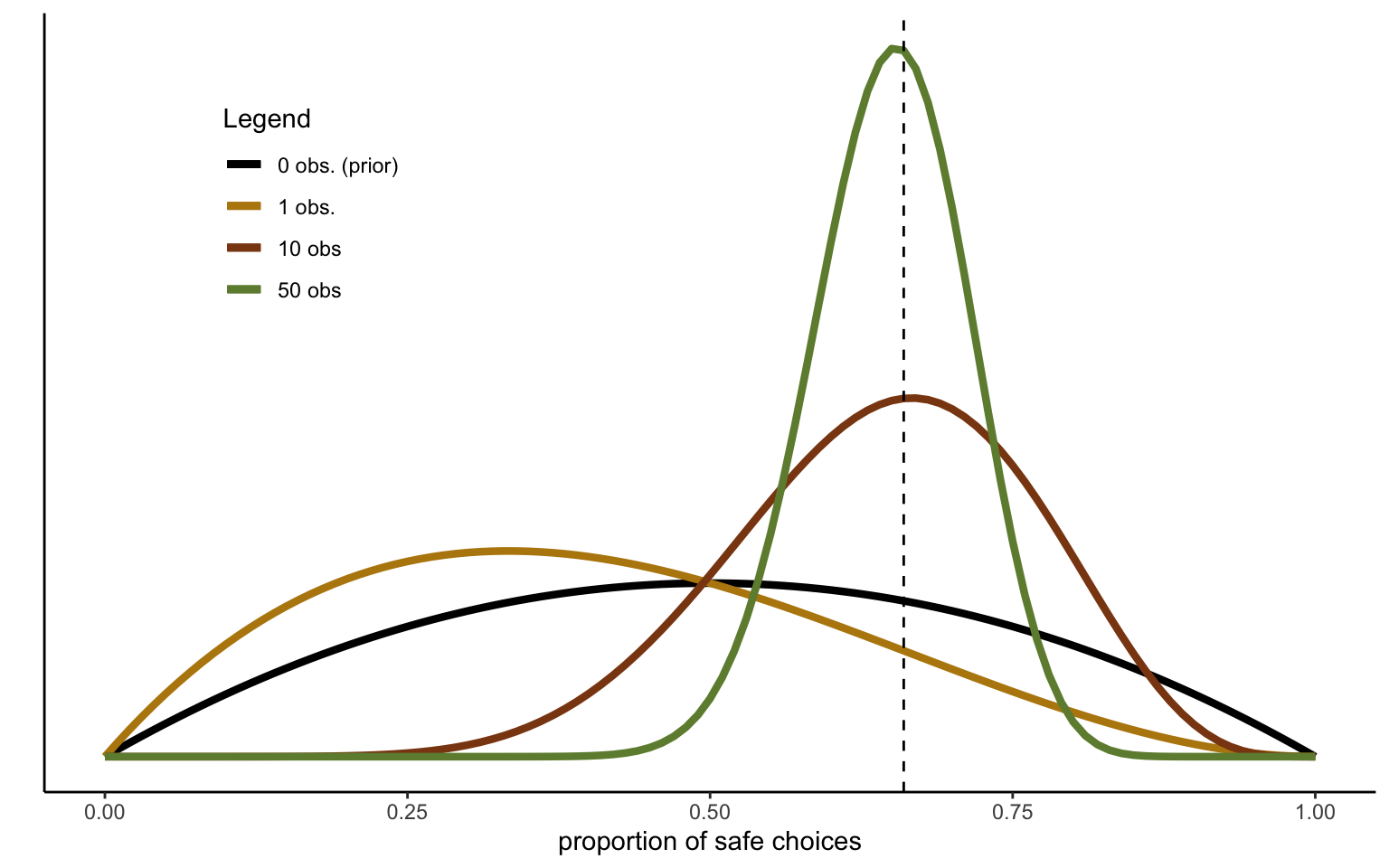
Figure 2.1: Sequentional Updating of Beta distribution.

Figure 2.1 shows the effect of sequentially updating a Beta prior with subsequent Bernoulli trials, simulated with a probability of 0.71 (and with a true sample average of 0.66 in the simulated data). The prior distribution \(\mathcal{B}e(2,2)\) is fairly diffuse, assigning nonzero probability mass to the whole probability space. It is also noninformative, being centered on an ignorance value of 0.5. That is, we do not make any strong assumptions a priori, centering the distribution on expected value maximization, and only making it mildly informative, in the sense that we slightly discount extreme values towards 0 or 1. Clearly, the initial updating can go in the wrong direction, depending on the luck of the draw, as is indeed the case in the example in the figure. Nevertheless, after 10 draws we are closing in on the true mean, and after 50 draws we identify the true mean with a fair degree of confidence. In this case, the result indicates a pronounced degree of risk aversion.

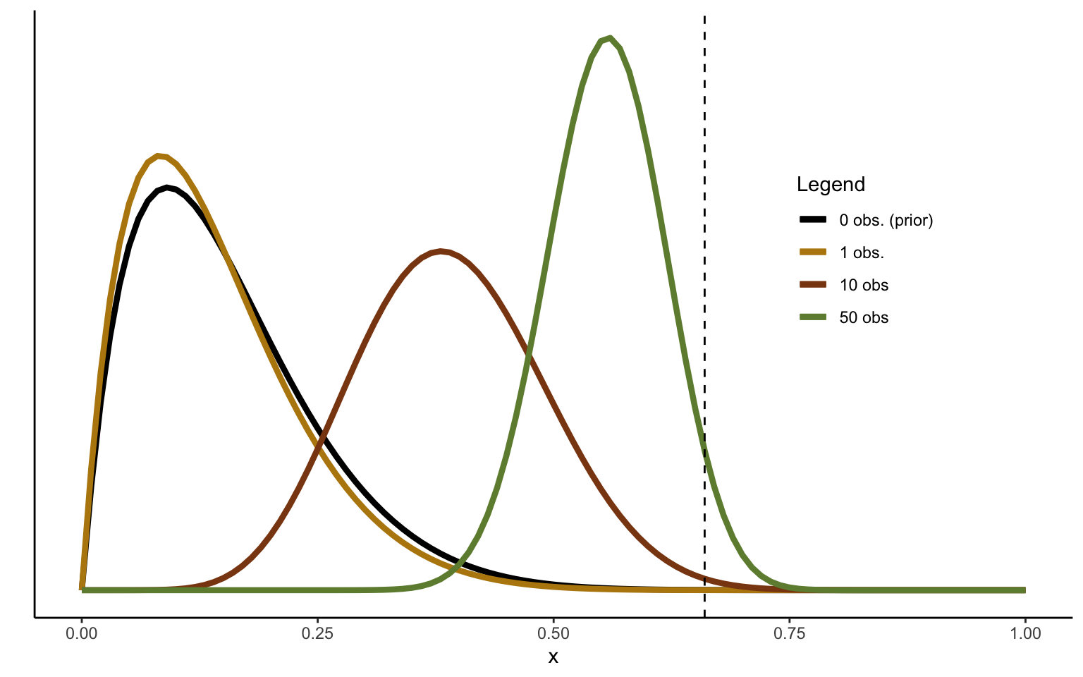
Of course, we may choose to use stronger priors, for instance because we know from many previous observations that subjects in similar tasks tend to be risk averse. Such a strategy could, for instance, be useful if we want to test risk aversion in several small groups drawn from the same population, and we want to avoid over-testing (we will discuss a more principled and better way of doing this in chapter III in the context of hierarchical analysis). For illustration purposes, however, let us assume that we expect the decision maker to be risk seeking, and that we are quite confident in this prior expectation to boot. Let us illustrate the effects of such an assumption with a Beta prior given by \(\mathcal{B}e(2,11)\), which indicates an expected outcome of \(\frac{2}{2 + 11} \approx 0.15\), and a fair degree of confidence in this estimate (the confidence in an estimate can be approximately indicated by the concentration of a Beta distribution, given by \(\alpha + \beta = 13\)).

set.seed(345678) 
obs <- rbernoulli(n=50,p=0.71) 
x <- append(obs,0,0)

alpha <- 2 
beta <- 11

for(i in 2:51){ alpha[i] <- alpha[i-1] + x[i]
                beta[i] <- beta[i-1] + (1 - x[i]) }

ggplot(data = data.frame(x = c(0, 1)), aes(x=x)) + stat_function(fun = dbeta, n = 101, args = list(shape1 = alpha[1], shape2 = beta[1]), size=1.5,aes(colour="0 obs. (prior)")) + 
  stat_function(fun = dbeta, n = 101, args = list(shape1 = alpha[2], shape2 = beta[2]), aes(colour="1 obs."),linewidth=1.5) + 
  stat_function(fun = dbeta, n = 101, args = list(shape1 = alpha[11], shape2 = beta[11]), aes(colour="10 obs"),linewidth=1.5) + 
  stat_function(fun = dbeta, n = 101, args = list(shape1 = alpha[51], shape2 = beta[51]), aes(colour="50 obs"),size=1.5) + 
  geom_vline(xintercept=mean(obs), aes(colour="red"), linetype="dashed") + 
  ylab("") + scale_y_continuous(breaks = NULL) + 
  scale_colour_manual("Legend", values = c("black","darkgoldenrod", "chocolate4", "darkolivegreen4")) + 
  theme(legend.position = c(0.8, 0.6))

Figure 2.2: Sequentional Updating of Beta distribution, strong prior.

Using the same simulations as used in Figure 2.1 above, we see from the distributions in Figure 2.2 that 50 observations are now no longer enough to converge to the sample mean—the pull of the prior is too strong. In general, the posterior will always lie between the prior and the maximum likelihood estimate in a Bayesian setup, although the Bayesian and ML estimates will converge as \(N\rightarrow \infty\). We can get a feel of this if we rewrite the updating equation with N observations as follows

\[\begin{align*} E(\theta|x) &= \frac{\alpha + m}{\alpha + \beta + N} \\ &= \frac{\alpha + m}{K + N} \\ &= \frac{K}{K + N}\frac{\alpha}{K} + \frac{N}{K + N}\frac{m}{N} \\ &= (1-\gamma) \frac{\alpha}{K} + \gamma \frac{m}{N}, \end{align*}\] where \(K \triangleq \alpha + \beta\) is the concentration. \(K\) then measures the “data points” contributed by the prior, while \(N\) measures the actual observations in the dataset as before. The parameter \(\gamma\) can then be taken as a measure of the shrinkage of the ML estimate \(\frac{m}{N}\) to the prior mean \(\frac{\alpha}{K}\). While priors can be a strength of the Bayesian approach, one ought to choose them carefully, since they may just as well distort one’s inferences from the data. In practice, it is thus always advisable to check the sensitivity of one’s results to a more diffuse prior, unless one has truly good reasons to adopt a particular prior distribution. We will discuss such cases in some detail in later parts of these notes.

2.2.2 Predictive distribution

Very often, we will want to predict new data based on past data. Note that the predictive distribution (also variously referred to as prior predictive or posterior predictive, depending on the use one makes of it and the last updating step) is generally not the same as the estimated posterior distribution. To predict future outcomes based on past data, we will want to integrate over the possible posterior parameter values, such that

\[\begin{align*} p(x_{N+1}|x) &= \int p(x_{N+1}|\theta) p(\theta | x) d\theta \\ &= \frac{\alpha + m}{\alpha + \beta + N}. \end{align*}\] That is, in the case of binary variables seen here, the predictive distribution is exceedingly simple, and coincides with the mean of the posterior. Note how the Bayesian approach can thus easily solve the issue arising from a series of four observations that all come up heads, as discussed above (aka black swan paradox). To solve this issue, simply assume a Beta prior with parameters \((1,1)\). The posterior predictive will be:

\[ p(x_{N+1}|x) = \frac{m + 1}{N + 2}. \]

This differs from 1 (and is also known as Laplace’s rule of succession, which has been used as a solution to the paradox in non-Bayesian approaches). Notice, however, that as we accumulate more and more observations pointing in the same direction that prediction will become quite extreme, albeit without every going to 0 or 1 entirely. (And of course in a Bayesian modl we could use values of \(\alpha\) and \(\beta\) different from 1, though we should be careful about what these parameters do and whether we are justified in choosing them).

2.3 Normal distribution

One of the most commonly used distributions in statistics is the normal, not least because of its computational tractability (but also because nature loves the normal distribution). Conveniently, the conjugate prior to the normal mean is itself normal, and their combination results in a normal posterior. In this section, I will first present the general underlying theory, and then develop some examples.

2.3.1 Likelihood and Prior

Take a dataset \(x = (x_1, …, x_n)\). We will ultimately want to infer the probability of some hypothesis or parameter, conditional on these data. To start, however, we can depict the probability of the data, given the parameters of the distribution, otherwise known as the likelihood:

\[ p(x|\mu,\sigma^2) = \frac{1}{\sqrt{2\pi}\sigma} exp\left(-\frac{1}{2\sigma^2}\sum_{i=1}^n (x_i - \mu)^2\right). \]

In Bayesian analysis, we will supplement this likelihood with a prior. It is important to note that, in Bayesian analysis, the data are always given, whereas it is the parameters that are uncertain. We thus want to use the known and given data to make inferences about the unknown and inherently uncertain parameters. Notice how this approach differs markedly from the assumption in classical or frequentist statistics, whereby parameters are given and certain but unknown to the statistician, and where we thus want to use random data samples to make inferences about these given but unknown parameters. In the latter, we could indeed use the sample quantities \(\overline{x} \triangleq \frac{1}{n}\sum_i x_i\) and \(s^2 \triangleq \frac{1}{n} \sum_i (x_i - \overline{x})^2\) to make inferences about the quantities \(\mu\) and \(\sigma\). Since theoretical occurrences from which the data are sampled are assumed to be infinite, our inferences should then be correct on average as long as we sample enough data (technically, in the limit as \(N \rightarrow \infty\)).

Since in the Bayesian setup the parameters \(\mu\) and \(\sigma\) are themselves uncertain, we can model them as being drawn from a distribution. One way to think about this is that, although we estimate them from the data at hand, they may still differ from the true underlying parameters due to sampling noise. If that is the case, we ought to be able to stabilize the estimates by bringing to bear any prior knowledge we may have about these parameters. In the presence of sampling noise, that is indeed a normative way of reining in the influence of noisy outliers. As we will see shortly, combination of empirical ML estimates with a prior will serve to draw the parameter estimates towards the prior in a precise and principled way. This is the origin of one of the great strengths of Bayesian statistics—its applicability to small samples.

Let us thus assume that the mean is drawn from the following prior distribution (we assume the sampling variance to be given for the time being):

\[ p(\mu|\mu_0,\sigma_0^2) = \frac{1}{\sqrt{2\pi}\sigma_0} exp\left(-\frac{1}{2\sigma_0^2}(\mu - \mu_0)^2\right), \] where I have written \(p(\mu|\mu_0,\sigma_0^2)\) to indicate the prior instead of \(p(\mu)\) to emphasize the dependency on the parameters governing the normal distribution.

We can think of this prior distribution as incorporating anything we know about the mean of similar data. This could for instance incorporate any theoretical insights we may have about the quantities, such that they will always be constrained to a certain range (unless, of course, our aim is to test that theory). Alternatively, one could think about the prior as being built over time from estimates of \(\mu\) obtained from similar datasets. Of course, we may then want to give a prior to the prior mean \(\mu_0\) itself, which is commonly referred to as a hyperprior. We will see in due time that meta-analysis may constitute a particularly principled way of building such a prior.

2.3.2 Bayesian updating with one datapoint

Let us assume for the moment that we only have one single data point, designated by \(x\) for simplicity. Throughout this section, we will also assume that the sample variance of this data point, \(\sigma^2\), is known. This may seem like an artificial assumption, but it will help us developing the framework step by step. Such sequential approaches are indeed important in practice, especially when it comes to machine learning and artificial intelligence (but also in computational neuroscience). Under these assumptions, it is now straightforward to derive the posterior expectation of the unknown and uncertain parameter \(\mu\) (the mean of the likelihood), conditional on the parameters of the prior: \[\begin{align*} \mathbb{E}[\, \mu \, | \, x ,\, \sigma ,\, \mu_0 ,\, \sigma_0 \, ] &= \frac{\sigma_0^2}{\sigma_0^2 + \sigma^2} \times x + \frac{\sigma^2}{\sigma_0^2 + \sigma^2}\times \mu_0 \\ &= \mu_0 + \frac{\sigma_0^2}{\sigma_0^2 + \sigma^2}(x - \mu_0) \\ &= x + \frac{\sigma^2}{\sigma_0^2 + \sigma^2}(\mu_0 - x). \end{align*}\] The three ways of writing the posterior expectation above highlight different intuitions about it. The first expression shows it as a convex combination between data point and prior mean; the second shows how the prior adjusts to the datapoint; and the third shows how the datapoint is drawn to the prior mean. This phenomenon in general is known as shrinkage or pooling, and it is a foundational concept in Bayesian statistics. For now, note that the degree of shrinkage is governed precisely by the ratio of variances: Shrinkage towards the mean of the prior is governed by the proportion of the total variance that is ascribed to sampling variation, \(\sigma^2\). Ceteris paribus, the larger the sampling noise, the more shrinkage to the prior mean. Mutatis mutandis, the adjustment of the prior mean to the data point will be larger the larger the uncertainty surrounding the prior mean itself. In the limit, as \(\sigma_0 \rightarrow \infty\), we can indeed see that the posterior mean converges to the maximum likelihood estimate. This is a useful result, since it implies that we can always recover the MLE estimate from Bayesian algorithms by imposing an (improper) prior with infinite variance.

Derivation of the normal updating equation

If you have never seen the equation above, you may wonder where it comes from. The result can be derived by multiplying the Gaussians describing the likelihood and prior to obtain the posterior, \(p(\mu | x) = p(x|\mu)\times p(\mu)\). To start let us write out the distributions (we drop the normalization constants, since these can easily be reinstated at the end): \[\begin{align*} p(x|\mu) &\propto exp\left(-\frac{1}{2} \frac{(x - \mu)^2}{\sigma^2}\right) \\ p(\mu) &\propto exp\left(-\frac{1}{2} \frac{(\mu - \mu_0)^2}{\sigma_0^2}\right) \end{align*}\] We next take logs to get rid of the exponentials, multiply out the squares, and group: \[\begin{align*} ln[p(\mu | x)] &\propto ln[p(x|\mu)] + ln[p(\mu)] \\ &\propto -\frac{1}{2} \frac{(x - \mu)^2}{\sigma^2} -\frac{1}{2} \frac{(\mu - \mu_0)^2}{\sigma_0^2} \\ &\propto -\frac{1}{2} \left(\frac{1}{\sigma^2} + \frac{1}{\sigma_0^2} \right)\mu^2 + \mu \left(\frac{x}{\sigma^2} + \frac{\mu_0}{\sigma_0^2} \right) - \left( \frac{x^2}{2\sigma^2} + \frac{\mu_0^2}{2\sigma_0^2} \right) \end{align*}\] The last step will be to “complete the square”. That is, we know that our log-posterior function will again be a Gaussian, so that it will take the following form: \[ ln[p(\mu | x)] = -\left(\frac{\mu^2}{2\sigma_p^2} - \frac{2\mu\mu_p}{2\sigma_p^2} + \frac{\mu_p}{2\sigma_p^2} \right), \] where \(\mu_p = \mathbb{E}[\, \mu \, | \, x ,\, \sigma ,\, \mu_0 ,\, \sigma_0 \, ]\) is the mean of the posterior distribution, and \(\sigma_p\) designates the variance of the posterior distribution. We can now match the first expression in the last equation above to the first expression in the last line of the previous equation: \[ -\frac{\mu^2}{2\sigma_p^2} = -\frac{1}{2} \left(\frac{1}{\sigma^2} + \frac{1}{\sigma_0^2} \right)\mu^2, \] which we solve for the variance of the posterior: \[ \sigma_p^2 = \frac{\sigma^2\sigma_o^2}{\sigma^2 + \sigma_o^2}. \] We then procced to matching the second term of the two equations: \[ - \frac{2\mu\mu_p}{2\sigma_p^2} = \mu \left(\frac{x}{\sigma^2} + \frac{\mu_0}{\sigma_0^2} \right). \] Solving for the mean of the poserior, we get: \[ \mu_p = \frac{\sigma_0^2}{\sigma_0^2 + \sigma^2} \, x + \frac{\sigma^2}{\sigma_0^2 + \sigma^2}\, \mu_0. \] While the calculations are tedious, there is clearly no magic involved.

Having obtained the posterior mean, we now also need to assess the variance surrounding the posterior mean. This will provide us with a direct measure of the uncertainty surrounding the estimate (NOTE: the standard deviation of the posterior in Bayesian analysis coincides with what is called a standard error in classical analysis). The variance of the posterior mean, conditional on the single data point being observed, will thus be:

\[ \mathbb{V}( \, \mu \, | \, x, \, \sigma , \, \sigma_0 ) = \frac{\sigma^2\sigma_0^2}{\sigma^2 + \sigma_0^2} = \frac{1}{\frac{1}{\sigma^2} + \frac{1}{\sigma_0^2}} \triangleq (\lambda + \lambda_0)^{-1}, \]

where \(\lambda \triangleq\sigma^{-2}\) is the precision of the likelihood, and \(\lambda_0 \triangleq \sigma_0^{-2}\) the precision of the prior. This notation is particularly intuitive, and it shows that the uncertainty surrounding the posterior will be inversely proportional to the sum of the precisions of the likelihood and the prior.

Let us discuss an example. Assume we have data made up of a collection of certainty equivalents (CEs), \(c =(c_1, … , c_n)\). Let us transform the CEs to indicate relative risk premia, \(r_i \triangleq p_i - \frac{c_i - y_i}{x_i - y_i}\). We want to find the average relative risk premium in the sample, \(\overline{r}\). We can simulate some data by drawing 50 observations from a distribution of relative risk premia, with a mean of 0.5 and a variance of about 0.1. Let us assume that we have a prior indicating that people are risk neutral on average, albeit with a fair degree of uncertainty \(p(\mu \,| \, \mu_0,\sigma_0^2) = \mathcal{N}(0 \, , \, 0.1)\). We can now take one data point at the time, and update this prior using the equation derived above. Note that the posterior resulting from the updating process with one data point can simply be taken to be the prior of the next iteration, thus nicely illustrating how information accumulates over time. Below, I do this starting from the first data point and following the sequence.

rrp <- rnorm(50,0.5,0.316)

lambda <- 1/var(rrp)
lambda0 <- 1/0.1
mu0 <- 0
x <- append(rrp,0,0)

for(i in 2:51){
lambda0[i] <- lambda0[i-1] + lambda
mu0[i] <- mu0[i-1] + (lambda)/(lambda + lambda0[i])*(x[i] - mu0[i-1])
}

ggplot(data = data.frame(x = c(-0.8, 0.8)), aes(x)) +
  stat_function(fun = dnorm, n = 101, args = list(mean = mu0[1], sd = sqrt(1/lambda0[1])), size=1.5,aes(colour="0 obs. (prior)")) +
  stat_function(fun = dnorm, n = 101, args = list(mean = mu0[2], sd = sqrt(1/lambda0[2])) ,size=1.5, aes(colour="1 obs.")) +
  stat_function(fun = dnorm, n = 101, args = list(mean = mu0[6], sd = sqrt(1/lambda0[6])), size=1.5, aes(colour="5 obs.")) +
  stat_function(fun = dnorm, n = 101, args = list(mean = mu0[11], sd = sqrt(1/lambda0[11])), size=1.5, aes(colour="10 obs.")) +
  stat_function(fun = dnorm, n = 101, args = list(mean = mu0[31], sd = sqrt(1/lambda0[31])), size=1.5, aes(colour="30 obs")) +
  geom_vline(xintercept=mean(rrp),linetype="dashed",colour="red", size=1.2) +
  ylab("")  + scale_y_continuous(breaks = NULL) +
  scale_colour_manual("Legend", values = c("black","darkgoldenrod", "chocolate4", "darkolivegreen4","steelblue3")) + theme(legend.position = c(0.1, 0.6))

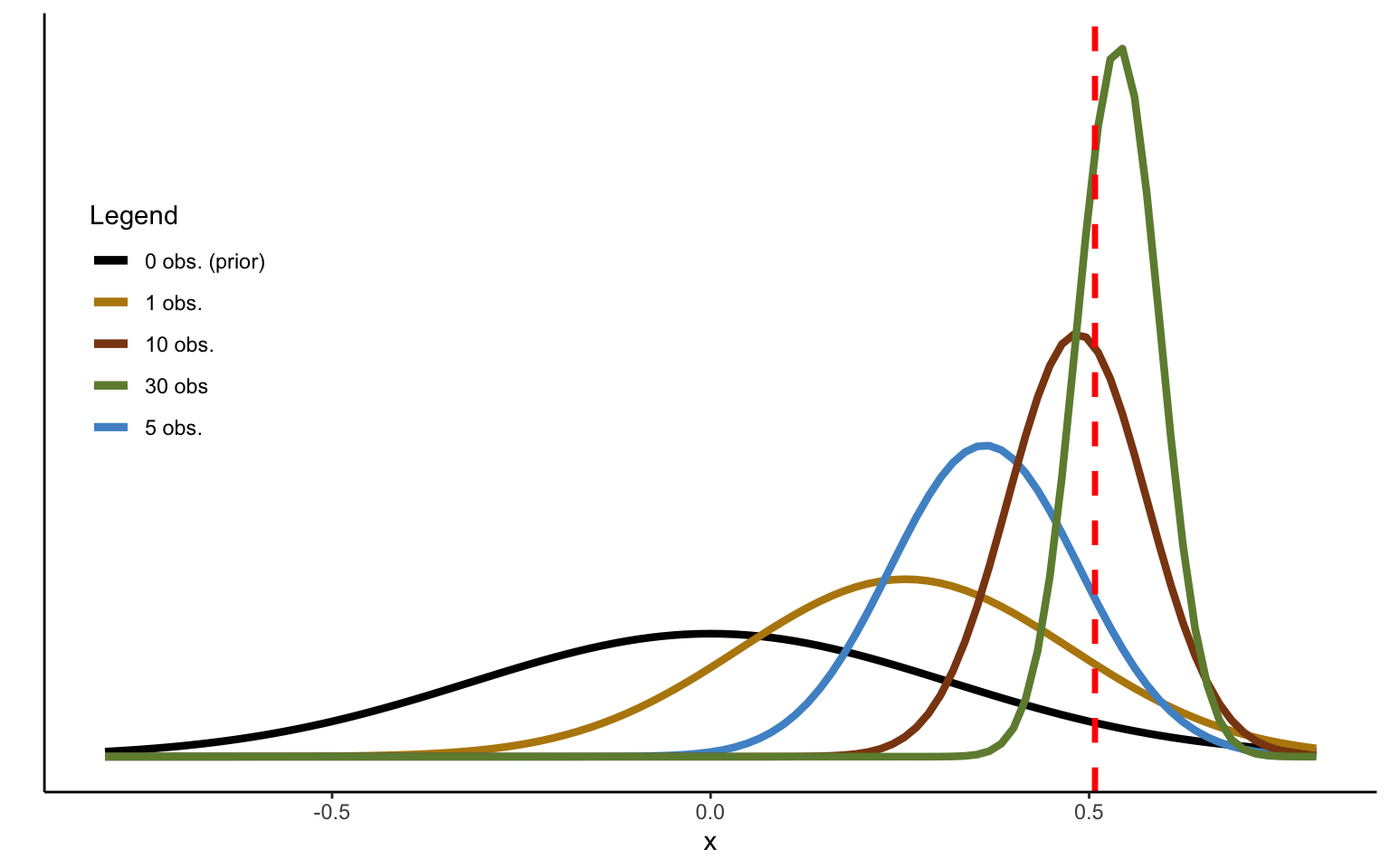
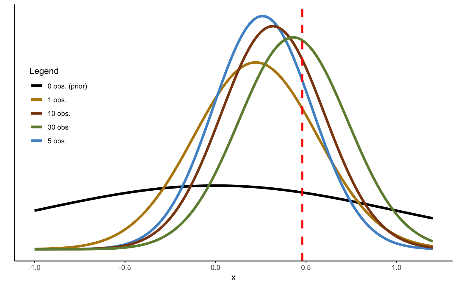
Figure 2.3: Sequentional Updating of Normal distribution.

The updating sequence in Figure 2.3 has been obtained by using the true sampling variance, and assuming it to be known. One can see that after 30 observations, the mean is learned almost perfectly and with a high degree of confidence. Note that while I start from prior parameters \(\mu_0\) and \(\lambda_0\), these are quickly updated to incorporate the information provided by the data, with the resulting posterior serving as the prior for the next observation.

2.3.3 Integrating several data points at once

Typically, we will want to combine several data points at once with the prior. Notice, however, that there is no difference between updating the prior with several data points at once or doing it sequentially. On the one hand, this makes it straightforward to derive the general case from the case seen above. On the other, this means that one could employ sequential methods if desirable, which may be interesting in learning algorithms and machine learning. In this section, I will show the equations needed to update the prior with several data points at once. Once again, it is assumed that the sampling variance is known.

Assuming that the observations in \(x\) are i.i.d., we know that the sample mean will follow the distribution \(p(\, \overline{x} \,| \,\mu \,) = \mathcal{N}(\,\mu \, ,\, \frac{\sigma^2}{n}\,)\). We can thus directly derive the posterior distribution as follows:

\[ p( \mu \, | \, x ) \sim \mathcal{N}\left(\frac{n\sigma_0^2}{n\sigma_0^2 + \sigma^2}\times \overline{x} + \frac{\sigma^2}{n\sigma_0^2 + \sigma^2} \mu_0 \enspace , \enspace (\lambda_0 + n\lambda)^{-1} \right). \]

Once again, we find shrinkage towards the mean of the prior, or a convex combination of sample mean and prior mean. Writing the updating equation for the mean as \(E[\mu|x] = \mu + \frac{\sigma_0^2}{\sigma_0^2 + \frac{\sigma^2}{n}}(\overline{x} - \mu)\) allows us to derive a number of interesting results. In the limit as \(n \rightarrow 0\) we simply revert to the mean of the prior. As \(n \rightarrow \infty\) the weight on the prior mean goes to zero. This shows that with enough data, the prior will be immaterial. It is for small datasets that the prior will be really important.

It is also instructive to look at the variance of the posterior in terms of precisions. This takes the following form:

\[ \mathbb{V}(\mu \,| \,x) = \frac{1}{\sigma_0^2} + \frac{n}{\sigma^2} = \lambda_0 + n\lambda. \]

Unsurprisingly, this is the same result we obtained above, when we added new observations one observation at a time, every time adding \(\frac{1}{\sigma^2}\) to the prior precision. It is interesting to see how the two precisions enter into the equation symmetrically. That is, for large \(n\) the posterior will depend mostly on \(\sigma^2\). For \(\sigma = \sigma_0\), as used in the illustration above, the prior will thus have the same weight as one extra observation with mean \(\mu_0\). This explains the quick convergence to the sample mean we observed in the simulated example above.

ggplot(data = data.frame(x = c(-1, 1)), aes(x)) +
  stat_function(fun = dnorm, n = 101, args = list(mean = 0, sd = 0.316), size=1.5) +
  stat_function(fun = dnorm, n = 101, args = list(mean = mu0[11], sd = sqrt(1/lambda0[11]) ) , colour="darkgoldenrod3",size=1.5) +
  stat_function(fun = dnorm, n = 101, args = list(mean = mean(head(rrp,n=10)), sd = (1/sqrt(10))*sd(head(rrp,n=10))),size=1.5,colour="darkolivegreen4") +
  ylab("")  + scale_y_continuous(breaks = NULL) +
  annotate(geom="text", x=-0.1, y=1.5, label="prior") +
  annotate(geom="text", x=0.3, y=4.5, label="N=10") +
  annotate(geom="text", x=0.7, y=1.3, label="likelihood") 

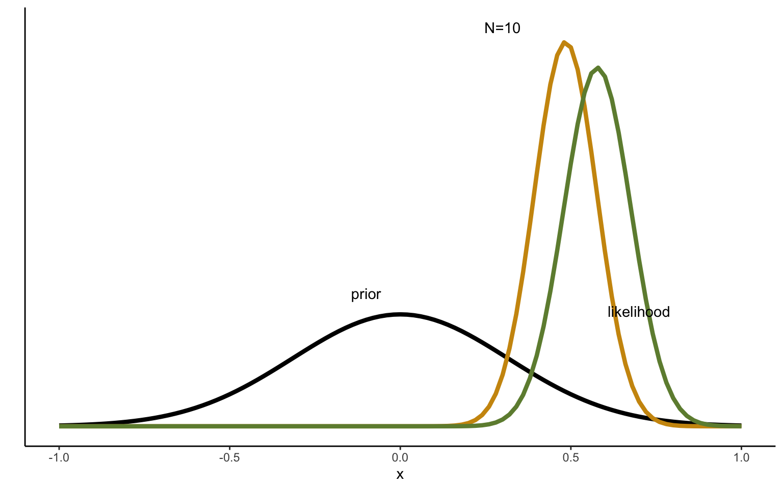
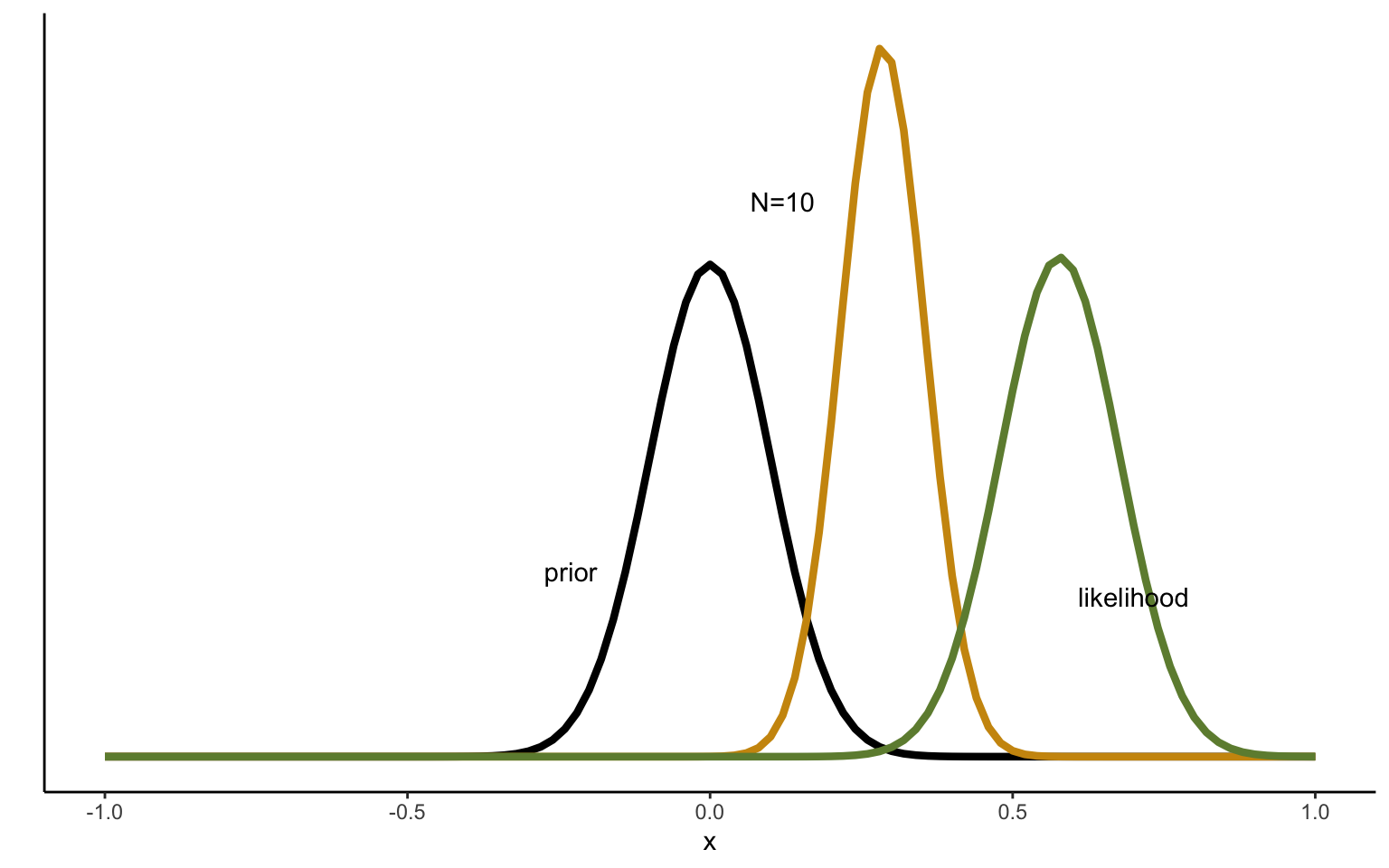
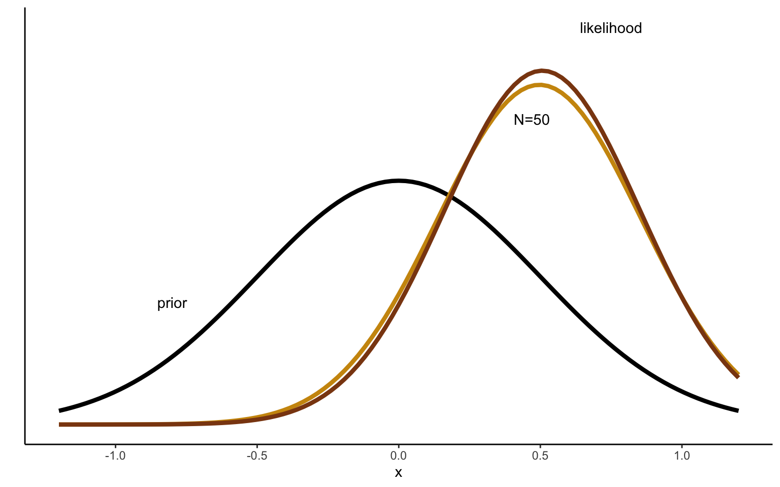
Figure 2.4: Sequentional Updating of Normal distribution with 10 draws.

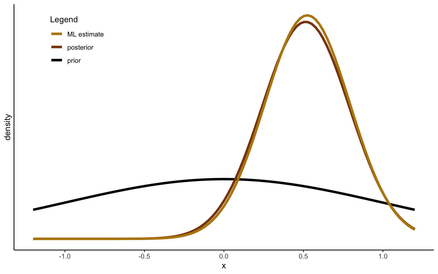
It may be interesting to take one more look at the effect of the prior with these insights in mind. We can use the same simulated data as above and take, say, the first 10 observations. We start by reproducing the graph above, but this time comparing the posterior distribution obtained after 10 draws to both the prior and to the maximum likelihood estimate, obtained based o the data alone. Figure 2.4 shows the result. We can see that the posterior, even after only 10 observations, is very close to the maximum likelihood estimate. In other words, the prior has fairly little influence in this example—one tenth of the evidence provided by the data to be exact.

lambda <- 1/var(rrp)
lambda0 <- 100
mu0 <- 0
x <- append(rrp,0,0)


for(i in 2:51){
lambda0[i] <- lambda0[i-1] + lambda
mu0[i] <- mu0[i-1] + (lambda)/(lambda + lambda0[i])*(x[i] - mu0[i-1])
}

ggplot(data = data.frame(x = c(-1, 1)), aes(x)) +
  stat_function(fun = dnorm, n = 101, args = list(mean = 0, sd = sqrt(1/lambda0[1])), size=1.5) +
  stat_function(fun = dnorm, n = 101, args = list(mean = mu0[11], sd = sqrt(1/lambda0[11])) , colour="darkgoldenrod3",size=1.5) +
  stat_function(fun = dnorm, n = 101, args = list(mean = mean(head(rrp,n=10)), sd = sqrt(1/10)*sd(head(rrp,n=10))),size=1.5,colour="darkolivegreen4") +
  ylab("")  + scale_y_continuous(breaks = NULL) +
  annotate(geom="text", x=-0.23, y=1.5, label="prior") +
  annotate(geom="text", x=0.12, y=4.5, label="N=10") +
  annotate(geom="text", x=0.7, y=1.3, label="likelihood") 

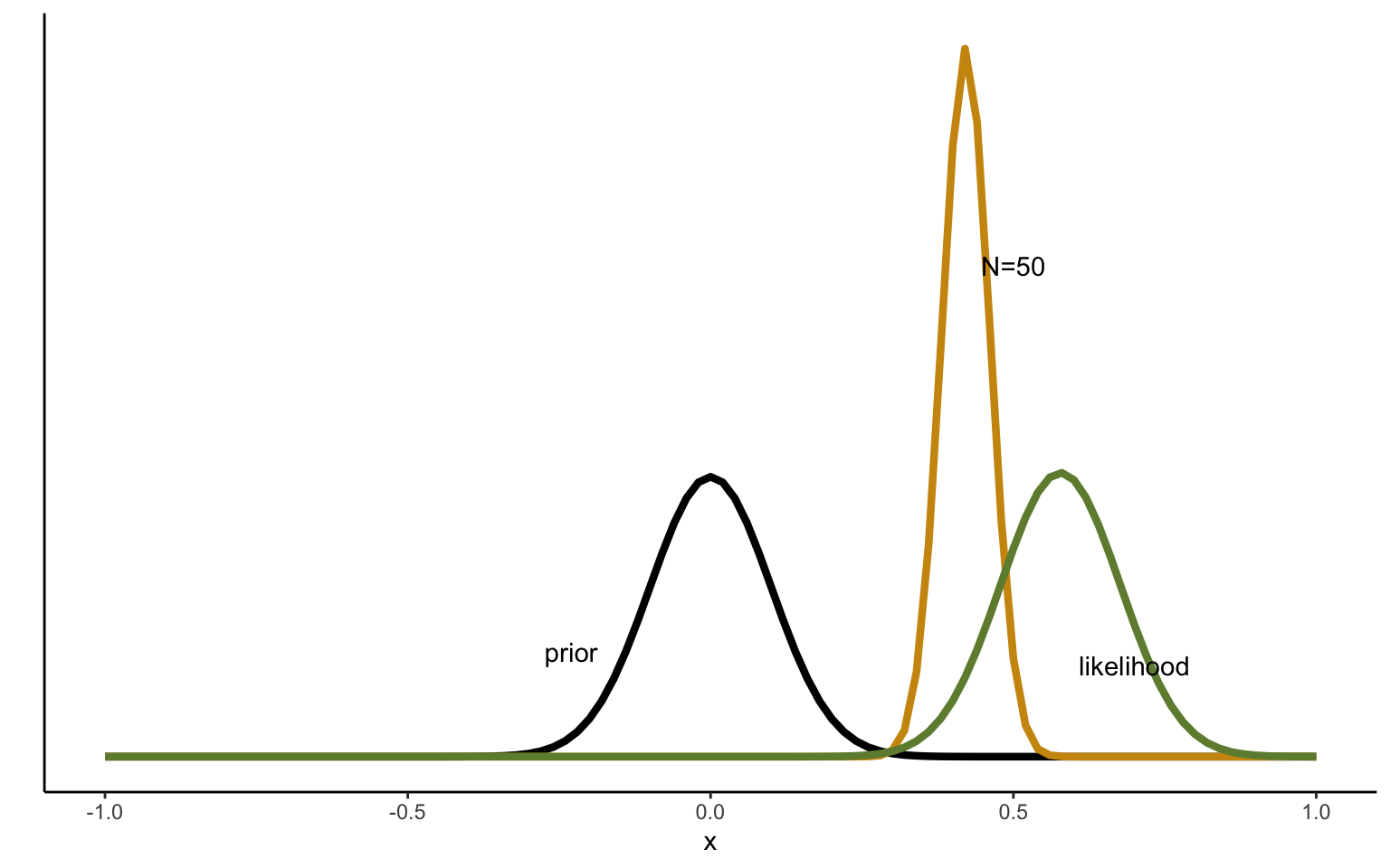
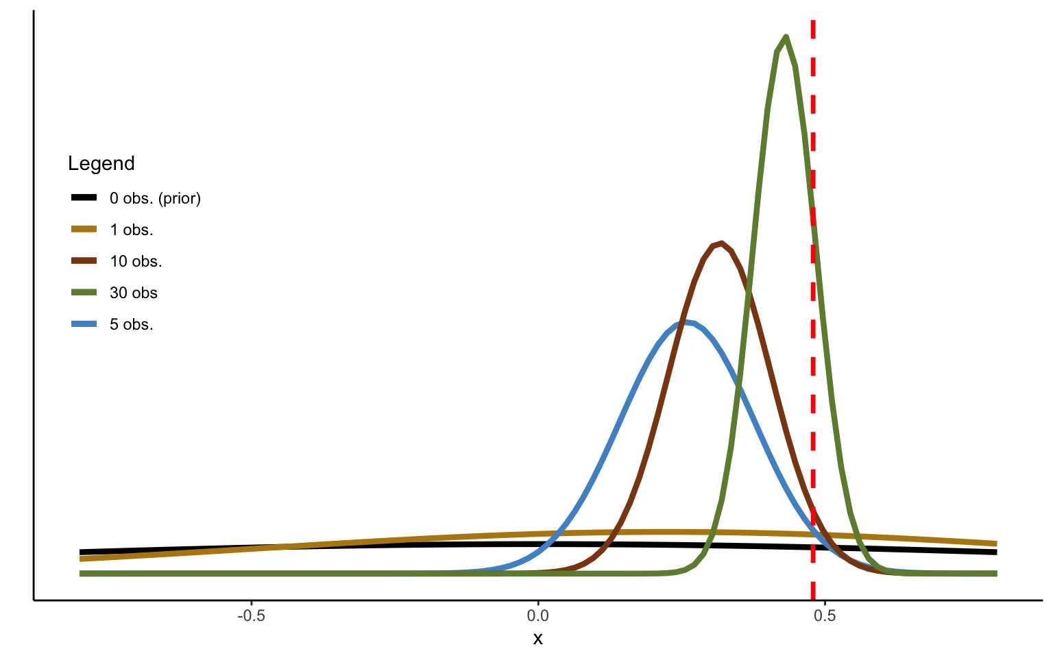
Figure 2.5: Sequentional Updating of Normal distribution, strong prior.

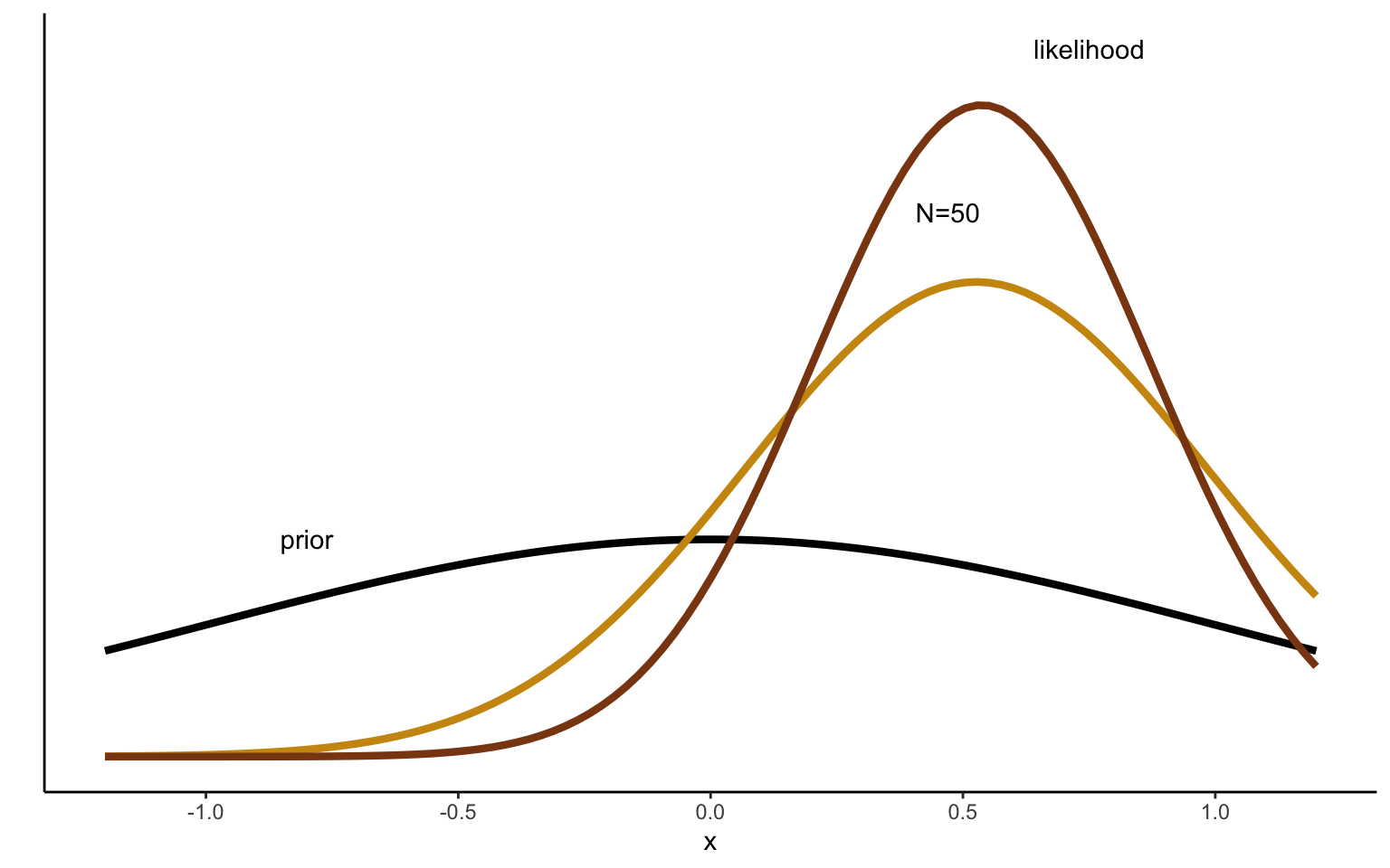
Next, we can repeat this exercise, but imposing a much narrower prior reflected by a large precision. The result is shown in Figure 2.5. We can see how the more precise prior exercises a stronger pull on the posterior estimate. Whereas the diffuse prior has little influence on the posterior even after 10 draws, resulting in a posterior distribution very close to the maximum likelihood estimate, the precise prior used just above means that the posterior mean estimated lands in the middle between the prior and the MLE.

Sequential updating is very natural in the Bayesian context, and can be put to use in contexts where it might be useful to learn gradually about the posterior. To see this more clearly, we can write the posterior as follows:

\[ p(\mu | x) \propto \left[ p(\mu) \prod_{i=1}^{n-1}p(x_i | \mu)\right]p(x_n|\mu), \]where the term in square brackets represents the posterior after \(n-1\) observations (which can be seen as a prior for observation \(n\)), and the last term to the right presents the contribution of the \(n^{th}\) observation. Notice also that we could now take the posterior obtained from the last sequential updating procedure above, and further update it with observations 11-50. I do not do this here for parsimony. Suffice it to say that, given the strength of the prior now imposed, even 50 observations are no longer enough for convergence to the ML estimate, as shown in Figure 2.6.

ggplot(data = data.frame(x = c(-1, 1)), aes(x)) +
  stat_function(fun = dnorm, n = 101, args = list(mean = 0, sd = sqrt(1/lambda0[1])), size=1.5) +
  stat_function(fun = dnorm, n = 101, args = list(mean = mu0[51], sd = sqrt(1/lambda0[51])) , colour="darkgoldenrod3",size=1.5) +
  stat_function(fun = dnorm, n = 101, args = list(mean = mean(head(rrp,n=10)), sd = sqrt(1/10)*sd(head(rrp,n=10))),size=1.5,colour="darkolivegreen4") +
  ylab("")  + scale_y_continuous(breaks = NULL) +
  annotate(geom="text", x=-0.23, y=1.5, label="prior") +
  annotate(geom="text", x=0.5, y=7, label="N=50") +
  annotate(geom="text", x=0.7, y=1.3, label="likelihood")

Figure 2.6: Sequentional Updating of Normal distribution with 50 draws, strong prior.

2.3.4 The posterior predictive distribution

We will often want to use the parameters obtained from past data to predict new data. For this, we need the posterior predictive distribution. Formally, we will want to predict observation(s) \(\tilde{x}\) from past observation(s) \(x\), so as to obtain \(p(\tilde{x}|x)\). For this, we will need to consider the likelihood of the new data, based on the parameters estimated on the old data

\[ p(\tilde{x} \, | \, x) \propto \int p(\tilde{x} \, | \, \mu) \, p(\mu \, | \, x) \, d\mu. \]

Note that the first distribution within the integral is just the likelihood, applied to the new data \(\tilde{x}\) we want to predict. The second distribution is the posterior distribution of \(\mu\), based on data \(x\). We do not need to condition the predicted quantity directly on past data, since the information they contain is fully reflected in this posterior. We need to integrate over all values of \(\mu\), because the posterior estimate of \(\mu\) is itself an uncertain quantity (i.e., it has a distribution). We can rewrite this equation as:

\[ p(\tilde{x}|x) \propto \int exp\left(-\frac{1}{2\sigma^2}(\tilde{x} - \mu)^2\right) exp\left(\frac{1}{2 \sigma_p^2}(\mu - \mu_p)^2 \right)d\mu, \]

where \(\mu_p \triangleq \mu_0 + \frac{\sigma_0^2}{\sigma_0^2 + \sigma^2}(x - \mu_0)\) and \(\sigma_p^2 \triangleq \frac{\sigma^2 \sigma_0^2}{\sigma^2 + \sigma_0^2}\) are the mean and variance of the posterior, respectively. It can then be shown that

\[\begin{align*} \mathbb{E}[\tilde{x}\, | \, x] &= \mu_p \\ \mathbb{V}[\tilde{x} \, | \, x] &= \sigma^2 + \sigma^2_p, \end{align*}\]

that is, the posterior predictive distribution will have a mean equal to the posterior mean based on \(x\), with a variance equal to the sum of the sampling variance and the posterior variance of the mean, which derives from uncertainty in the estimation of \(\mu_p\).

2.3.5 Conjugate priors for the variance

We have now seen how to infer the value of the mean when the variance is known. However, the variance will not be known in general, and we will thus need to make inferences about the variance of the sampling distribution. To simplify things, we will assume for the time being that the mean is known, and that we are trying to infer only the variance, making this the dual situation of the one seen above.

While different parametrizations are used in the literature, I will work with a prior for the precision, \(\lambda \triangleq \frac{1}{\sigma^2}\). The likelihood function then takes the following form: \[\begin{align*} p(x \, | \, \lambda) &= \prod_{i=1}^n \mathcal{N}(x_i|\mu,\lambda^{-1}) \\ &\propto \lambda^{\frac{1}{2}}exp\left[-\frac{\lambda}{2} \sum_{i=1}^n(x_i - \mu)^2\right]. \end{align*}\]

Given the above formulation in terms of precision, the conjugate prior will take the form of a Gamma distribution, defined as follows: \[ Gam(\lambda | \alpha , \beta) = \frac{1}{\Gamma(\alpha)}\beta^\alpha\lambda^{\alpha - 1}exp(-\beta \lambda), \] where \(\Gamma(\alpha)\) is a Gamma function which serves to normalize the distribution.

Assume now a prior distribution \(Gam(\lambda | \alpha_0,\beta_0)\). Multiplying this with the likelihood function above we obtain a posterior distribution, which, conveniently, again follows a Gamma: \[ p(\lambda | D) \propto \lambda^{\alpha_0 - 1} \lambda^\frac{N}{2} exp\left[-\beta_0 \lambda - \frac{\lambda}{2} \sum_{i=1}^{n}(x_i - \mu)^2\right], \] which we can designate as \(Gam(\lambda | \alpha_n , \beta_n)\). We can thus write the updating equations as follows: \[\begin{align*} \alpha_n &= \alpha_0 + \frac{n}{2} \\ \beta_n &= \beta_0 + \frac{1}{2}\sum_{i=1}^{n}(x_i - \mu)^2 \\ &= \beta_0 + \frac{n}{2} s^2, \end{align*}\] where \(s^2\) is the maximum likelihood estimate of the variance in the data. Note that the normalization factor \(\Gamma(\alpha)\) can be found easily in the end, so that there is no need to keep track of it during the updating process. We can easily see that \(n\) data points increase the coefficient \(\alpha\) by \(\frac{n}{2}\). It follows immediately that one data point increases it by \(\frac{1}{2}\). The parameter \(\beta\), on the other hand, is increased proportionally to the squared deviation from the mean. Since the mean of a Gamma distribution is \(\mathbb{E}[\lambda] = \frac{\alpha}{\beta}\), the crucial element for the evolution of the precision will be which of the two parameters increases more quickly. The variance of the precision is defined as \(\mathbb{V}[\lambda] = \frac{\alpha}{\beta^2}\).

rrp <- rnorm(50,0.5,0.316)
lambda <- 1/var(rrp)
alpha <- 1
beta <- 1
x <- append(rrp,0,0)

for(i in 2:51){
alpha[i] <- alpha[i-1] + 0.5
beta[i] <- beta[i-1] + 0.5*(x[i] - mean(rrp))^2
}

ggplot(data = data.frame(x = c(0, 20)), aes(x)) +
  stat_function(fun = dgamma, args = list(shape = alpha[1], rate=beta[1]), size=1.5,aes(colour="0 obs. (prior)")) +
  stat_function(fun = dgamma, args = list(shape = alpha[2], rate=beta[2]), size=1.5, aes(colour="1 obs.")) +
  stat_function(fun = dgamma, args = list(shape = alpha[6], rate=beta[6]), size=1.5, aes(colour="5 obs.")) +
  stat_function(fun = dgamma, args = list(shape = alpha[11], rate=beta[11]), size=1.5, aes(colour="10 obs.")) +
  stat_function(fun = dgamma, args = list(shape = alpha[51], rate=beta[51]), size=1.5, aes(colour="50 obs.")) +
  geom_vline(xintercept=1/var(rrp),colour="red",linetype="dashed") +
  ylab("") + xlab("precision")  + scale_y_continuous(breaks = NULL) +
  scale_colour_manual("Legend", values = c("black","darkgoldenrod", "chocolate4", "darkolivegreen4","steelblue3")) + theme(legend.position = c(0.8, 0.7))

Figure 2.7: Sequential updating of precision.

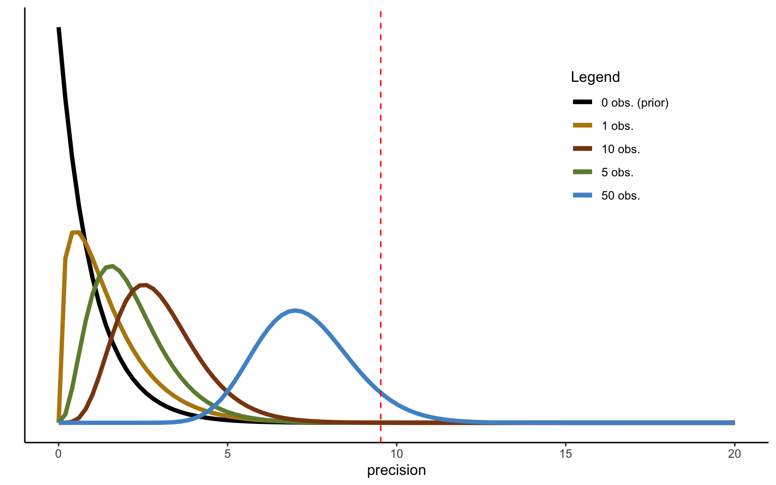
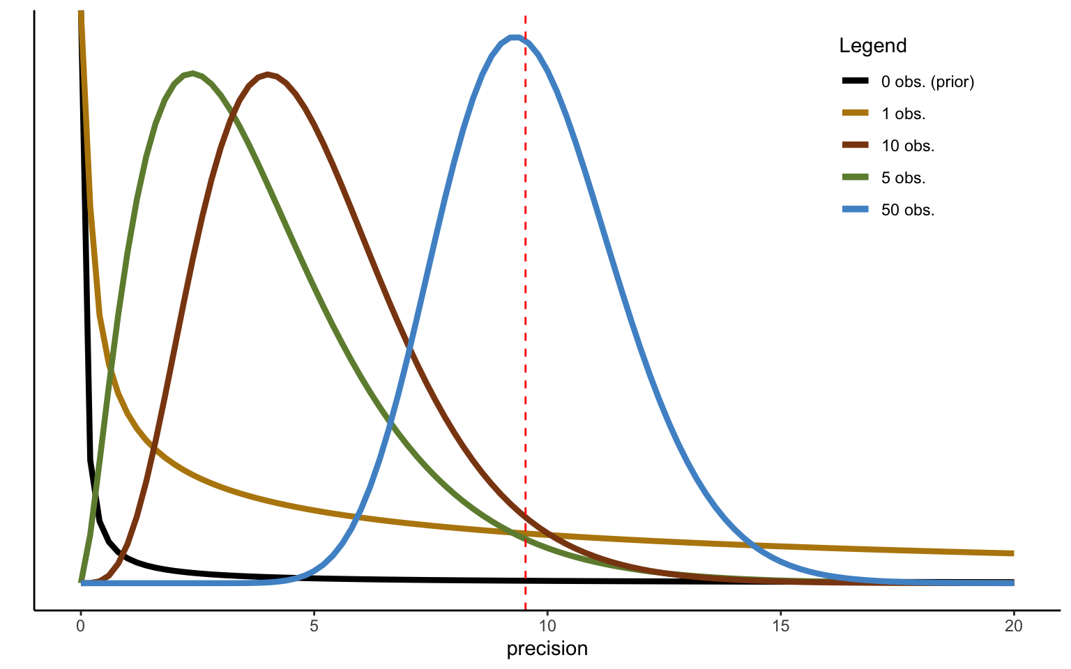
This updating process can thus be implemented in a sequential fashion. Let us again consider an example. We start from a prior with parameters \(\alpha_0 = 1\) and \(\beta_0 = 1\), and we can use the same data of relative risk premia generated above. The result of the updating process is depicted in Figure 2.7. Convergence to the true mean now seems very slow, and even after 50 observations the posterior estimate is still far from the sample mean, indicated by the vertical dashed line. What has happened? A quick examination of the parameters used above will tell you that this is due to the high probability mass assigned to very low precision levels in the prior we have used. In particular, the prior distribution used has a mean of 1 (compared to a sampling mean of the precision of 12.55), as well as a variance of 1, indicating high confidence in the (unrealistic) prior mean of the precision.

alpha <- 1
beta <- 0.1
x <- append(rrp,0,0)

for(i in 2:51){
alpha[i] <- alpha[i-1] + 0.5
beta[i] <- beta[i-1] + 0.5*(rrp[i-1] - mean(rrp))^2
}

ggplot(data = data.frame(x = c(0, 20)), aes(x)) +
  stat_function(fun = dgamma, args = list(shape = alpha[1], rate=beta[1]), size=1.5,aes(colour="0 obs. (prior)")) +
  stat_function(fun = dgamma, args = list(shape = alpha[2], rate=beta[2]), size=1.5, aes(colour="1 obs.")) +
  stat_function(fun = dgamma, args = list(shape = alpha[6], rate=beta[6]), size=1.5, aes(colour="5 obs.")) +
  stat_function(fun = dgamma, args = list(shape = alpha[11], rate=beta[11]), size=1.5, aes(colour="10 obs.")) +
  stat_function(fun = dgamma, args = list(shape = alpha[51], rate=beta[51]), size=1.5, aes(colour="50 obs.")) +
  geom_vline(xintercept=1/var(rrp),colour="red",linetype="dashed") +
  ylab("") + xlab("precision")  + scale_y_continuous(breaks = NULL) +
  scale_colour_manual("Legend", values = c("black","darkgoldenrod", "chocolate4", "darkolivegreen4","steelblue3")) +
  theme(legend.position = c(0.85, 0.8))

Figure 2.8: Sequential updating of precision, weak prior.

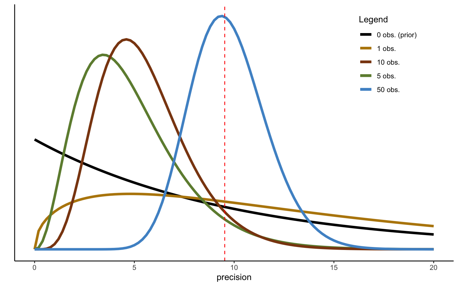
To convince yourself of this, try using a more diffuse prior. The distributions shown in Figure 2.8 do just this, by using a shape parameter of \(\alpha_0 = 1\) for the prior as before, but a much lower rate parameter \(\beta_0 = 0.1\). Note that this will have two effects. The mean of the prior, defined as \(\frac{\alpha_0}{\beta_0} = 10\) is now much larger. At the same time, the variance, defined as \(\frac{\alpha_0}{\beta_0^2} = 100\), makes the prior much more diffuse. Convergence to the sample variance is now much quicker, and the estimated mean (of the variance) coincides with the sample mean after 50 iterations/data points (though the mode falls slightly to the left of it—keep in mind that the distribution is not symmetric).

alpha <- 0.01
beta <- 0.01

for(i in 2:51){
alpha[i] <- alpha[i-1] + 0.5
beta[i] <- beta[i-1] + 0.5*(rrp[i-1] - mean(rrp))^2
}

ggplot(data = data.frame(x = c(0, 20)), aes(x)) +
  stat_function(fun = dgamma, args = list(shape = alpha[1], rate=beta[1]), size=1.5,aes(colour="0 obs. (prior)")) +
  stat_function(fun = dgamma, args = list(shape = alpha[2], rate=beta[2]), size=1.5, aes(colour="1 obs.")) +
  stat_function(fun = dgamma, args = list(shape = alpha[6], rate=beta[6]), size=1.5, aes(colour="5 obs.")) +
  stat_function(fun = dgamma, args = list(shape = alpha[11], rate=beta[11]), size=1.5, aes(colour="10 obs.")) +
  stat_function(fun = dgamma, args = list(shape = alpha[51], rate=beta[51]), size=1.5, aes(colour="50 obs.")) +
  geom_vline(xintercept=1/var(rrp),colour="red",linetype="dashed") +
  ylab("") + xlab("precision")  + scale_y_continuous(breaks = NULL) +
  scale_colour_manual("Legend", values = c("black","darkgoldenrod", "chocolate4", "darkolivegreen4","steelblue3")) + 
  theme(legend.position = c(0.85, 0.8))

Figure 2.9: Sequential updating of precision, ceteris paribus.

You may well consider this example as cheating. After all, we have not only increased the variance to 100, making the prior more diffuse, but we have also adjusted the mean to 10, bringing it very close to the sample mean, and thus making it informative. Alternatively, one could thus try and keep the mean constant at a low level, while only allowing the variance to increase. Figure 2.9 shows an example doing exactly that. I have now set both the shape and the rate parameters to 0.1. This implies a mean of the precision equal to 1, as in the first example above, but a variance equal to 100, like in the second example above. Convergence to the sample mean is once again complete after 50 data points, thus showing that the result was driven mostly by the diffuseness of the prior (the larger variance), and not by the higher mean.

2.3.6 Conjugate priors: learning mean and variance together

We have now seen how to update the mean of the normal distribution with new information, as well as how to update the variance. An intuitive conclusion would seem that we can simply put the two steps together to update mean and variance at once, and to thus learn the entire distribution. This intuition, however, is only partially correct. The additional issue arising when updating both parameters at once is that, conditional on the data, they are not independent from each other (to convince yourself of this, simply take a look at the functional form of the normal distribution). Ignoring this dependence would imply that the prior is not conjugate after all.

The solution turns out to be a prior that follows a so-called normal-gamma distribution, and indicated as \(\mathcal{NG}(\mu_0,\kappa_0,\alpha_0,\beta_0)\). Assume as usual that the probability of the data conditional on the parameters follows a normal distribution, so that \(p(x_i|\mu,\lambda) = \mathcal{N}(\mu,\lambda^{-1})\). Note that I have now conditioned the probability of the data explicitly on both the mean and the variance (actually: the precision), since both are now assumed unknown. We now want to identify a joint prior for the two unknown model parameters. To do this, we can exploit the fact that \(p(\mu,\lambda) = p(\mu | \lambda) \, p(\lambda)\). As it turns out, \(p(\lambda)\) will again take the form of a Gamma distribution, whereas \(p(\mu | \lambda)\) will take the form of a normal. The dependency between the parameters is then captured by making the precision of the conditional distribution of the mean a linear function of \(\lambda\): \[ p(\mu,\lambda) = \mathcal{N}(\mu|\mu_0,(\kappa_0\lambda)^{-1}) \, Gam(\lambda|\alpha_0,\beta_0), \] where \(\beta_0\) is again the rate parameter of the Gamma distribution. The scaling parameter \(\kappa_0\) drives home the dependency between the different parameters, and expresses the precision of the prior relative to the precision of the data. To better understand this, it is instructive to take a look at the updating equations. I here start from an update with \(n\) observations. Let us start from the equation for the mean conditional on data \(x = (x_1, ... , x_n)\) and on the precision:

\[\begin{align} \mathbb{E}[\mu|x,\lambda] &=\frac{n\lambda}{n\lambda + \kappa_0\lambda} \overline{x} + \frac{\kappa_0\lambda}{n\lambda + \kappa_0\lambda}\mu_0 \\ &= \mu_0 + \frac{n\lambda}{n\lambda + \kappa_0\lambda} (\overline{x} - \mu_0) \\ &= \mu_0 + \frac{n}{n + \kappa_0} (\overline{x} - \mu_0), \end{align}\] where \(\overline{x} \triangleq \frac{1}{n}\sum_i^n x_i\). Notice that this equation is equivalent to the one used previously, with two differences. For one, I have expressed the updating weights in terms of precisions instead of in terms of variances. To see the equivalence, let \(\kappa_0\lambda = \frac{1}{\sigma_0^2}\) and \(n\lambda = \frac{1}{\sigma^2}\). Then \(\frac{n\lambda}{n\lambda + n_0\lambda} = \frac{\frac{1}{\sigma^2}}{\frac{1}{\sigma^2} + \frac{1}{\sigma_0^2}} = \frac{\sigma_0^2}{\sigma_0^2 + \sigma^2}\). The second and more substantive change consists precisely in the reparameterization of the prior precision as \(\kappa_0\lambda\). The scaling parameter \(\kappa_0\) serves to fix the relative strength of the prior. The updating equation for the variance of the mean will then simply be as follows:

\[ \mathbb{V}(\mu|x) = (n\lambda + \kappa_0\lambda)^{-1}. \]

The equations just described are conditional not only on the data \(x\), but also on the precision \(\lambda\). We thus still need to consider the probability of \(\lambda\), \(p(\lambda|x)\). We already know that this equation will take the form of a Gamma. To obtain the posterior estimates of the parameters of this distribution, in the case of an n-dimensional data vector we can use the following updating equations:

\[\begin{align*} \alpha_n &= \alpha_0 + \frac{n}{2} \\ \beta_n &= \beta_0 + \frac{1}{2}\sum_{i=1}^{n}(x_i - \mu)^2 \\ &= \beta_0 + \frac{1}{2}\sum_{i=1}^{n}(x_i - \overline{x})^2 + \frac{1}{2}\frac{n \kappa_0}{n + \kappa_0}(\overline{x} - \mu_0)^2) \\ \kappa_n &= \kappa_0 + n, \end{align*}\] where the last expression to the right in the middle equation obtains from taking into account the expression for \(\mu\) above. That is, since both \(\mu\) and \(\lambda\) need to be learned from the data and the dependence of both on \(x\) creates inter-dependencies between the variables, only an equation system explicitly taking account of these inter-dependencies will yield the desired results. In terms of interpretation, it is easy to see that the \(\beta\) value of the posterior will depend both on the variance of the data sample, \(\sum_{i=1}^{n}(x_i - \overline{x})^2\), and on the deviation of the sampling mean from the prior mean, \((\overline{x} - \mu_0)^2\). The weight of the latter, in turn, will depend on the supposed `number of observations’ in each.

Simulations will serve to shed some light on the working mechanism of the equations. Some issues need to be kept in mind. First of all, while we have started from the probability of the mean conditional on the precision, we now need to work in the opposite direction. Finally, one needs to take good care not to get confused between the different variables—both mean and variance will have a posterior mean and a posterior variance of their own!

rrp <- rnorm(50,0.5,0.316)

n <- length(rrp)
mu0 <- 0
alpha <- 0.01
beta <- 0.01
k0 <- 1

alpha_n <- alpha + n/2
beta_n <- beta + 0.5*sum((rrp - mean(rrp))^2) + (n*k0)/(2*(n + k0)) * (mean(rrp) - mu0)^2
mu <- mu0 + (n)/(n  + k0) * (mean(rrp) - mu0)
k_n = k0 + n
lambda <- alpha_n/beta_n
lambda_n <- k_n*lambda

# learned distribution compared to prior and ML estimate:
ggplot(data = data.frame(x = c(-1.2, 1.2),y=c(0,0.2)), aes(x)) +
  stat_function(fun = dnorm, n = 101, args = list(mean = mu0, sd = (k0*(alpha/beta))^(-0.5) ), size=1.5,aes(colour="prior")) +
  stat_function(fun = dnorm, n = 101, args = list(mean = mu, sd = sqrt(lambda^(-1))) ,size=1.5,aes(colour="posterior")) +
  stat_function(fun = dnorm, n = 101, args = list(mean = mean(rrp), sd = (sd(rrp))) , size=1.5,aes(colour="ML estimate")) +
  scale_colour_manual("Legend", values = c("darkgoldenrod", "chocolate4","black", "darkolivegreen4","steelblue3")) +
 scale_y_continuous(breaks = NULL) +
theme(legend.position = c(0.15, 0.85)) +
 labs(y="density",x="x")

Figure 2.10: Batch updating of normal mean and variance.

Let us start from a prior centered at \(\mu_0\), and with \(\alpha_0 = \beta_0 = 0.1\), yielding a diffuse uninformative Gamma prior for the precision. We set \(\kappa_0 = 1\), given the precision prior a low weight corresponding to just 1 observation. The convergence to the sample distribution, shown in Figure 2.10, is almost complete (notice how I have plotted the learned posterior distribution, instead of the posterior of the mean, which has precision \(\lambda_n\)). In terms of the variance, this is due to the very diffuse albeit uninformative prior. For the mean, however, the low value of \(\kappa_0\) is crucial. We can think of this as virtual draws from our prior, or in other words, of the confidence we have in the prior itself. It is easy to show that increasing this parameter will result in a more precise prior, and consequently in increased shrinkage towards the prior mean. Figure 2.11 does just that. By increasing the weight on the prior to \(\kappa_0 = 10\), the prior becomes much more precise, and convergence to the likelihood after integrating 50 data points is thus much less complete.

rrp <- rnorm(50,0.5,0.316)

n <- length(rrp)
mu0 <- 0
alpha <- 0.01
beta <- 0.01
k0 <- 10

alpha_n <- alpha + n/2
beta_n <- beta + 0.5*sum((rrp - mean(rrp))^2) + (n*k0)/(2*(n + k0)) * (mean(rrp) - mu0)^2
mu <- mu0 + (n)/(n  + k0) * (mean(rrp) - mu0)
k_n = k0 + n
lambda <- alpha_n/beta_n
lambda_n <- k_n*lambda

# learned distribution compared to prior and ML estimate:
ggplot(data = data.frame(x = c(-1.2, 1.2),y=c(0,0.2)), aes(x)) +
  stat_function(fun = dnorm, n = 101, args = list(mean = mu0, sd = (k0*(alpha/beta))^(-0.5) ), size=1.5) +
  stat_function(fun = dnorm, n = 101, args = list(mean = mu, sd = sqrt(lambda^(-1))) ,
  colour="darkgoldenrod3",size=1.5) +
  stat_function(fun = dnorm, n = 101, args = list(mean = mean(rrp), sd = (sd(rrp))) , colour="chocolate4",size=1.5) +
  ylab("")  + scale_y_continuous(breaks = NULL) +
  annotate(geom="text", x=-0.23, y=1.25, label="prior") +
  annotate(geom="text", x=0.47, y=1, label="N=50") +
  annotate(geom="text", x=0.75, y=1.3, label="likelihood") 

Figure 2.11: Batch updating of normal mean and variance.

rrp <- rnorm(50,0.5,0.316)

n <- length(rrp)
mu0 <- 0
alpha <- 3
beta <- 3
k0 <- 1

alpha_n <- alpha + n/2
beta_n <- beta + 0.5*sum((rrp - mean(rrp))^2) + (n*k0)/(2*(n + k0)) * (mean(rrp) - mu0)^2
mu <- mu0 + (n)/(n  + k0) * (mean(rrp) - mu0)
k_n = k0 + n
lambda <- alpha_n/beta_n
lambda_n <- k_n*lambda

# learned distribution compared to prior and ML estimate:
ggplot(data = data.frame(x = c(-1.2, 1.2),y=c(0,0.2)), aes(x)) +
  stat_function(fun = dnorm, n = 101, args = list(mean = mu0, sd = (k0*(alpha/beta))^(-0.5) ), size=1.5) +
  stat_function(fun = dnorm, n = 101, args = list(mean = mu, sd = sqrt(lambda^(-1))) ,
  colour="darkgoldenrod3",size=1.5) +
  stat_function(fun = dnorm, n = 101, args = list(mean = mean(rrp), sd = (sd(rrp))) , colour="chocolate4",size=1.5) +
  ylab("")  + scale_y_continuous(breaks = NULL) +
  annotate(geom="text", x=-0.8, y=0.4, label="prior") +
  annotate(geom="text", x=0.47, y=1, label="N=50") +
  annotate(geom="text", x=0.75, y=1.3, label="likelihood") 

Figure 2.12: Batch updating of normal mean and variance.

It is also interesting to see what happens if one plays around with the parameters of the precision prior. In Figure 2.12 I have set the weight on the prior back to 1, i.e. \(\kappa_0 = 1\). I have, however, increased both the shape and rate parameters of the Gamma prior, to \(\alpha_0 = \beta_0 = 3\). Note that the mean of the prior precision remains unaffected at \(\frac{\alpha_0}{\beta_0} = 3\). What changes, however, is the variance of the precision, which becomes very small at \(\frac{\alpha_0}{\beta_0^2} = \frac{1}{3}\), making the prior of the precision, well, more precise. We can now see that the posterior precision is shrunk towards the variance of the prior. The effect, shown in the graph, is that the mean still converges to the mean of the data, but we have now much less confidence in this estimate. This is the effect of the strong prior put on the precision, as explored in detail in the previous section, when displayed in the form of the posterior inference on the normal distribution.

2.3.7 Sequential updating

An interesting special case of the equations above obtains in the case of sequential updating with 1 observation at the time, i.e. updating subsequently with every arrival of a new \(x_i\). Notice how only the squared deviation from the prior mean is of importance now, since \(x_i = \overline{x}\). The sample variance will thus be made up by a single squared deviation from the prior mean in each case. As the sample mean is updated and learned from observation to observation, we will furthermore need to adjust the scaling parameter, which I will now refer to as \(\kappa_i\). The updating equations for the prior will thus become:

\[\begin{align*} \alpha_i &= \alpha_{i-1} + \frac{1}{2}\\ \beta_i &= \beta_{i-1} + \frac{1}{2}\frac{\kappa_{i-1}}{\kappa_{i-1} + 1}(x_i - \mu_{i-1})^2 \\ \mu_i &= \mu_{i-1} + \frac{1}{\kappa_{i-1} + 1}(x_i - \mu_{i-1}) \\ \kappa_i &= \kappa_{i-1} + 1 \\ \tau_i &= \lambda_i + \kappa_i \lambda_i. \end{align*}\]

rrp <- rnorm(50,0.5,0.316)
x <- append(rrp,0,0)

alpha <- 0.01
k <- 1
beta <- 0.01
mu <- 0
lambda <- alpha/beta
lambda_m <- alpha/beta

for(i in 2:51){
alpha[i] <- alpha[i-1] + 1/2
beta[i] <- beta[i-1] + (k[i-1])/(2*(k[i-1] + 1)) * (x[i] - mu[i-1])^2
mu[i] <- mu[i-1] + (1)/(1  + k[i-1]) * (x[i] - mu[i-1])
k[i] <- k[i-1] + 1
lambda[i] <- alpha[i]/beta[i]
lambda_m[i] <- lambda[i-1] + k[i-1] * lambda[i-1]
}


# learned distribution compared to prior and ML estimate:
ggplot(data = data.frame(x = c(-1, 1.2)), aes(x)) +
  stat_function(fun = dnorm, n = 101, args = list(mean = mu[1], sd = sqrt(1/lambda[1])), size=1.5,aes(colour="0 obs. (prior)")) +
  stat_function(fun = dnorm, n = 101, args = list(mean = mu[2], sd = sqrt(1/lambda[2])) ,size=1.5, aes(colour="1 obs.")) +
  stat_function(fun = dnorm, n = 101, args = list(mean = mu[6], sd = sqrt(1/lambda[6])), size=1.5, aes(colour="5 obs.")) +
  stat_function(fun = dnorm, n = 101, args = list(mean = mu[11], sd = sqrt(1/lambda[11])), size=1.5, aes(colour="10 obs.")) +
  stat_function(fun = dnorm, n = 101, args = list(mean = mu[31], sd = sqrt(1/lambda[31])), size=1.5, aes(colour="30 obs")) +
  geom_vline(xintercept=mean(rrp),linetype="dashed",colour="red", size=1.2) +
  ylab("")  + scale_y_continuous(breaks = NULL) +
  scale_colour_manual("Legend", values = c("black","darkgoldenrod", "chocolate4", "darkolivegreen4","steelblue3")) + theme(legend.position = c(0.1, 0.6))

Figure 2.13: Sequential updating of normal mean and variance.

Figure 2.13 shows the sequential updating starting from a diffuse noninformative prior. After about 30 observations, both the mean and variance are (almost) perfectly learned under this parametrization. Alternatively, we can take a look at the posterior for the mean, i.e. incorporating the precision of the mean instead of the sampling distribution, shown in Figure 2.14. The mean estimate converges to the sampling estimate fairly quickly, just like shown above. The major difference now is that the precision surrounding the mean becomes ever larger, and the distribution hence more concentrated. That is indeed what should happen—as we add observations, our confidence in the mean estimate will grow progressively larger.

ggplot(data = data.frame(x = c(-0.8, 0.8)), aes(x)) +
  stat_function(fun = dnorm, n = 101, args = list(mean = mu[1], sd = sqrt(1/lambda_m[1])), size=1.5,aes(colour="0 obs. (prior)")) +
  stat_function(fun = dnorm, n = 101, args = list(mean = mu[2], sd = sqrt(1/lambda_m[2])) ,size=1.5, aes(colour="1 obs.")) +
  stat_function(fun = dnorm, n = 101, args = list(mean = mu[6], sd = sqrt(1/lambda_m[6])), size=1.5, aes(colour="5 obs.")) +
  stat_function(fun = dnorm, n = 101, args = list(mean = mu[11], sd = sqrt(1/lambda_m[11])), size=1.5, aes(colour="10 obs.")) +
  stat_function(fun = dnorm, n = 101, args = list(mean = mu[31], sd = sqrt(1/lambda_m[31])), size=1.5, aes(colour="30 obs")) +
  geom_vline(xintercept=mean(rrp),linetype="dashed",colour="red", size=1.2) +
  ylab("")  + scale_y_continuous(breaks = NULL) +
  scale_colour_manual("Legend", values = c("black","darkgoldenrod", "chocolate4", "darkolivegreen4","steelblue3")) + theme(legend.position = c(0.1, 0.6))

Figure 2.14: Sequential updating of normal mean and precision.

2.3.8 An alternative parametrization

We have now seen how to obtain the mean and variance by modelling the mean conditional on the precision. In some cases, however, it may be convenient to work with the variance directly. This could be done using an inverse-Gamma distribution. A more intuitive parametrization, however, can be obtained by means of a scaled inverse-Chi squared, which I will write \(\chi^{-2}\). Once again, we will factorize the joint prior distribution, \(p(\mu,\sigma^2) = p(\sigma^2)p(\mu|\sigma^2)\). The two distributions take the following form:

\[\begin{align*} p(\mu|\mu_0,\sigma^2/\kappa_0) &= \mathcal{N} \left(\mu_0, \frac{\sigma^2}{\kappa_0} \right)\\ p(\sigma^2/\nu_0,\sigma_0) &= \chi^{-2}(\nu_0,\sigma_0^2). \end{align*}\]

The basic setup is thus similar to the one seen above. The main difference consists in the use of the Chi-2, which is parameterized using degrees of freedom \(\nu_0\) and the variance of the prior \(\sigma_0^2\).

Assume you observe \(n\) data points \(x=(x_1,...,x_n)\). Then the posterior distribution will again take the form of a normal-Chi-square distribution, \(N\chi^{-2}(\mu,\sigma^2|\mu_n,\sigma^2_n/\kappa_n,\nu_n,\sigma^2_n)\). The updating equations will look as follows: \[\begin{align*} \mu_n &= \mu_0 + \frac{n}{\kappa_0 + n}(\overline{x} - \mu_0) \\ \kappa_n &= \kappa_0 + n \\ \nu_n &= \nu_0 + n \\ \sigma_n^2 &= \frac{1}{\nu_n}\left(\nu_0 \sigma_0^2 + \sum_i(x_i - \overline{x})^2 + \frac{\kappa_0 n}{\kappa_0 + n}(\overline{x} - \mu_0)^2 \right),\\ \tau_i &= \frac{\nu_0}{\sigma_0^2} + \frac{\kappa_0}{\sigma_0^2} \end{align*}\] where the posterior degrees of freedom are thus given by the prior degrees of freedom plus the sample size. It is left as an exercise to show that this parametrization produces results identical to those obtained above based on the normal-gamma prior. Results based on sequential updating are shown in Figure 2.15.

rrp <- rnorm(50,0.5,0.316)

k0 <- 1
nu0 <- 1
mu0 <- 0
sigma0 <- 0.5

n <- length(rrp)
sm <- mean(rrp)
sq <- sum((rrp - sm)^2)

mu <- mu0 + (n/(n+k0))*(sm - mu0)
k <- k0 + n
nu <- nu0 + n
sigma <- 1/nu * (nu0*sigma0 + sq + (k0*n/(k0+n)) * (sm - mu0)^2 )
tau <- nu0/sigma0 + k0/sigma0
  
  
ggplot(data = data.frame(x = c(-1.2, 1.2),y=c(0,0.2)), aes(x)) +
  stat_function(fun = dnorm, n = 101, args = list(mean = mu0, sd = (sigma0/k0) ), size=1.5) +
  stat_function(fun = dnorm, n = 101, args = list(mean = mu, sd = sqrt(sigma)) ,
  colour="darkgoldenrod3",size=1.5) +
  stat_function(fun = dnorm, n = 101, args = list(mean = mean(rrp), sd = (sd(rrp))) , colour="chocolate4",size=1.5) +
  ylab("")  + scale_y_continuous(breaks = NULL) +
  annotate(geom="text", x=-0.8, y=0.4, label="prior") +
  annotate(geom="text", x=0.47, y=1, label="N=50") +
  annotate(geom="text", x=0.75, y=1.3, label="likelihood")   

Figure 2.15: Sequential updating of normal mean and precision.

2.4 Conclusion

We have now examined some simple cases of conjugate updating. While more general analysis will require the use of simulation algorithms, these simple cases nevertheless help developing intuition for some of the fundamental processes at work. They are also very useful if one wants to use back-of-the-envelop calculations to obtain quick but exact estimates of the posterior under different assumptions about the prior, albeit at the cost of having to assume specific distributional forms.